7 Euclidean shapes and Deligne–Mostow periods

7.1 The fixed-curvature leaf at the Euclidean end

Fix $n\ge4$ and real numbers $$0<\mu_i<1,\qquad \sum_{i=1}^n\mu_i=2.$$(7.1) The Euclidean cone opening at the $i$th marked point is $2\pi(1-\mu_i)$, so $2\pi\mu_i$ is its curvature deficit. A conformal sphere $X$ with these marked points carries a unique such flat metric up to multiplication by a positive constant. In a coordinate with all marks finite it has the explicit form $$g_{\mathrm E,\mu}=C\prod_i|w-p_i|^{-2\mu_i}|\mathop{}\!\mathrm dw|^2.$$(7.2) The sum condition makes infinity a regular point. Near $p_i$, radial integration gives a cone of opening $2\pi(1-\mu_i)$. Thus the space of oriented, labeled Euclidean cone spheres with these deficits, up to similarity, has underlying complex manifold $\mathcal M_{0,n}$.

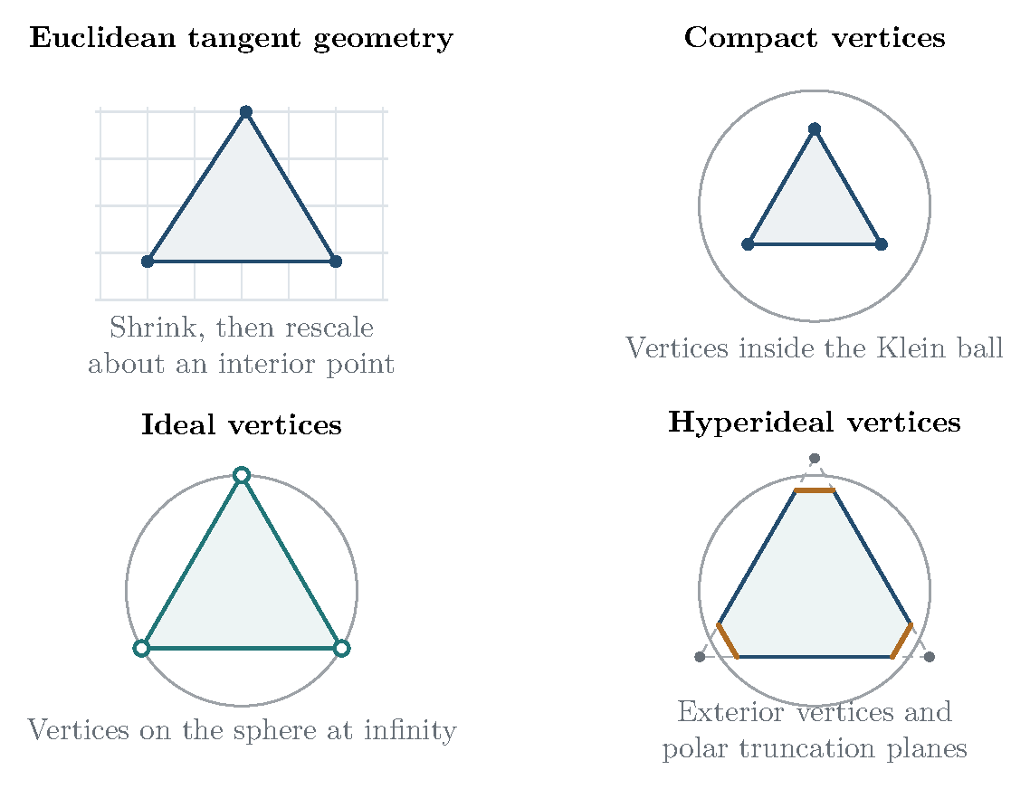
Alexandrov realization identifies these metrics with convex Euclidean polyhedral surfaces, allowing doubled planar polygons. This is the fixed-deficit space on which Thurston constructs his complex hyperbolic metric [97; 57]. The qualification “fixed deficits” is essential: all Euclidean polyhedra with $n$ vertices, up to similarity, form a space of real dimension $3n-7$, whereas the fixed-deficit leaf has real dimension $2n-6$. The full space of compact hyperbolic $n$-vertex polyhedra has dimension $3n-6$; its fixed-cone-angle leaves again have dimension $2n-6$. The ideal locus has dimension $2n-6$. These dimension counts apply on the generic strata; changes of combinatorics and flattened realizations require the usual cell structure. Figure 2 distinguishes these geometric regimes and the rescaled Euclidean limit.

7.2 The same periods describe hypergeometric functions and developed edges

Define the multivalued differential $$\eta_p(w)=\prod_i(w-p_i)^{-\mu_i}\,\mathop{}\!\mathrm dw.$$(7.3) Its branches differ by unit complex numbers. It therefore defines a twisted cohomology class for a rank-one unitary local system on the punctured sphere. The relevant twisted cohomology space has complex dimension $n-2$, and its Hermitian intersection form $H$ has signature $(1,n-3)$, with the convention that the class of $\eta_p$ has positive norm. In a local basis of twisted cycles or regularized relative arcs, the coordinates $$Z_j(p)=\int_{\gamma_j}\eta_p$$(7.4) are the hypergeometric periods of Deligne–Mostow [53]. Projectivizing their positive line gives a local map to $\mathbb{CH}^{n-3}$. Analytic continuation produces projective unitary monodromy.

Thurston’s Euclidean construction uses exactly the same coordinates. The local developing map is $$F(w)=\int^w\eta_p.$$ Hence a developed edge vector is an integral of $\eta_p$ along the corresponding arc. Cutting along a tree produces a Euclidean polygon whose edge vectors are periods, and whose area is the Hermitian form in these periods. Normalize $H$ by this area pairing. Then, more intrinsically, $$\mathcal A(p)=\frac{i}{2}\int_{\mathbb P^1}\eta_p\wedge\overline{\eta_p} =H(Z(p),Z(p)).$$(7.5) Multiplication of all periods by a nonzero complex number changes only the scale and rotation of the developed surface. Quotienting by this action is precisely the projectivization in the Deligne–Mostow construction.

Thus the connection is an equality of geometric structures: the hypergeometric periods are the developed edge vectors, and the Hermitian intersection pairing is the area pairing. Kojima proves that the two constructions, with labels retained, are canonically isometric [66, Lemmas 4.1–4.2 and Theorem 4.3]. The scalar used for the Hermitian intersection pairing varies between sources; fixing it by (7.5) removes that ambiguity, and a constant scalar does not change the projective metric. Throughout this monograph the complex hyperbolic metric has holomorphic sectional curvature $-1$. Its Kähler form, in the preceding local period coordinates, is $$\omega_{\mathrm{CH}}=-2i\,\partial\bar\partial\log\mathcal A.$$(7.6) A holomorphic change of local scale for $\eta_p$ does not affect this form. On a complex line in the ball, $\mathcal A=1-|z|^2$ gives $\mathop{}\!\mathrm ds^2=4|\mathop{}\!\mathrm dz|^2/(1-|z|^2)^2$, which checks the curvature normalization directly. A curvature-$-4$ convention would divide the form by $4$ and the volume in complex dimension $d$ by $4^d$.

If the weights are rational, choose their least common denominator $q$, so $\mu_i=m_i/q$. The compact normalization of the connected cyclic cover $$y^q=\prod_i(w-p_i)^{m_i}$$ makes $\eta_p=\mathop{}\!\mathrm dw/y$ a single-valued holomorphic differential. Under the deck transformation $y\mapsto e^{2\pi i/q}y$ it has eigenvalue $e^{-2\pi i/q}$. The corresponding eigenspace in the ordinary cohomology of this cover realizes the twisted cohomology. This gives a further useful interpretation in terms of periods of algebraic curves; it does not require the monodromy group to be a lattice.

7.3 Collision angles and the lattice conditions

Suppose two marks of total weight $\mu_i+\mu_j<1$ collide, with local separation $\delta$, while the other marks remain distinct and away from the collision. After fixing a branch, rescaling the integration variable in their vanishing period gives $$Z_{ij}(\delta)=C\delta^{\,1-\mu_i-\mu_j}(1+O(\delta)),\qquad C\ne0.$$(7.7) The transverse complex hyperbolic cone angle is consequently $2\pi(1-\mu_i-\mu_j)$. Deligne–Mostow’s condition INT is $$(1-\mu_i-\mu_j)^{-1}\in\mathbb Z_{>0} \quad\text{for every pair with }\mu_i+\mu_j<1.$$(7.8) Under this condition the completion by finite-distance collisions has orbifold universal cover $\mathbb{CH}^{n-3}$, and the monodromy is a lattice. Cusps remain at infinite distance. For the half-integral variant, fix a block of equal-weight marks and permit every permutation within that block. Interchanging two of its marks sends $\delta$ to $-\delta$; the quotient coordinate is $\delta^2$, so the transverse angle is halved. Mostow’s $\Sigma$INT condition is therefore $$(1-\mu_i-\mu_j)^{-1}\in \begin{cases} \tfrac12\mathbb Z_{>0},&i,j\text{ both in the specified block},\\ \mathbb Z_{>0},&\text{otherwise}, \end{cases} \qquad \mu_i+\mu_j<1.$$ Mostow’s theorem gives an orbifold uniformization for that permutation quotient [81, Sections 1–3]; the labeled completion need not itself be an orbifold when a reciprocal is a nonintegral half-integer. Thurston gives the corresponding criterion when all equal-weight permutations are allowed [97, Theorem 0.2].

When $\mu_i+\mu_j=1$, the collision is a cusp rather than a finite cone-angle divisor; logarithmic periods and parabolic monodromy enter. For general real weights satisfying (7.1), the local complex hyperbolic geometry and its finite volume still exist [97, Theorem 0.2]. One must not infer a lattice quotient for arbitrary weights. Conversely, INT and $\Sigma$INT are the classical sufficient uniformization conditions, not a claim to classify every exceptional discrete hypergeometric monodromy group. Our volumes retain all labels; a quotient by allowed equal-weight permutations changes the quotient and the volume factors.

7.4 Four equal deficits and elliptic periods

For $n=4$ and $\mu_i=1/2$, put the marks at $0,1,z,\infty$. Then $$\eta=\frac{\mathop{}\!\mathrm dw}{\sqrt{w(w-1)(w-z)}},\qquad E_z:\ y^2=w(w-1)(w-z).$$(7.9) The Euclidean cone sphere is the flat pillowcase quotient of this elliptic curve. The ratio of two periods gives a coordinate $\tau\in\mathbb H$. For $0<z<1$, one choice is $$\tau(z)=i\frac{K(1-z)}{K(z)},\qquad K(z)=\int_0^{\pi/2}\frac{\mathop{}\!\mathrm du}{\sqrt{1-z\sin^2u}}.$$(7.10) Here $z$ is the elliptic parameter, not its square root. The inverse map is the modular lambda function. Projective monodromy is $\mathrm P\Gamma(2)=\Gamma(2)/\{\pm I\}$, and the labeled moduli space is the thrice-punctured sphere with curvature-$-1$ area $2\pi$. The action of $S_4$ on the cross-ratio has the Klein four-group as its kernel. Its effective quotient therefore has degree $6$, and is the modular orbifold of area $\pi/3$; dividing the labeled area by $24$ would instead retain the ineffective stabilizer [66, Example 2.1 and Section 5]. This is the flat endpoint of the equal-angle torus–sphere correspondence in Section 6.