16 Dehn filling, variational response, and quantum surgery

16.1 Peripheral conventions and the two small parameters

Let $M$ be an oriented, finite-volume, one-cusped hyperbolic three-manifold. Fix an oriented meridian–longitude basis $(\mu,\lambda)$ and the geometric deformation branch through the complete structure. We use logarithms of the $\mathrm{PSL}_2(\mathbb C)$ multipliers, equivalently of the eigenvalue ratios, so that $$u=H(\mu),\qquad v=H(\lambda),\qquad v(u)=\tau u+c_3u^3+c_5u^5+O(u^7),\qquad B=\Im\tau>0.$$(16.1) Thus $u$ is twice a local logarithm of an $\mathrm{SL}_2$ eigenvalue, after removing its constant sign at the complete representation. In particular, the smooth filling equation is $pu+qv=2\pi i$, with the branch chosen continuously from the cusp. Using eigenvalue logarithms $\widehat u=u/2$, $\widehat v=v/2$ instead gives $p\widehat u+q\widehat v=\pi i$ and $\widehat v=\tau\widehat u+4c_3\widehat u^3+16c_5\widehat u^5+\cdots$. The oddness and the holomorphic potential are those of Neumann–Zagier [36, Sections 4–6].

For a primitive slope $(p,q)$ put $$A=p+q\tau,\qquad Q(p,q)=\frac{|A|^2}{B},\qquad pu+qv(u)=i\theta.$$(16.2) Here $\theta$ is an angular holonomy parameter. It is the cone angle when the local structure has the corresponding geometric cone completion; $\theta=0$ is the complete cusp and $\theta=2\pi$ gives a smooth hyperbolic filling when that completion exists. The quantity $Q$ is the squared length of the slope on a Euclidean cusp cross section divided by its area. For sufficiently long slopes the small solution stays in one fixed holonomy neighborhood throughout $0\leq\theta\leq2\pi$. Indeed, put $h(u)=v(u)-\tau u=O(u^3)$ and $t=q/A$. Since $|t|\leq B^{-1}$, a sufficiently small disk has $|t h'(u)|<1/2$ uniformly in the slope. The equation $u+t h(u)=i\theta/A$ then has a unique small analytic solution, uniformly for bounded $\theta$ and sufficiently large $|A|$, with $u=O(|A|^{-1})$. This is an assertion about a holonomy germ; the hyperbolic Dehn surgery theorem supplies the smooth geometric completion for sufficiently long primitive slopes [36, Section 4]. Geometric completion is a separate statement from the analytic existence of this small solution.

Two expansions must be kept distinct: $|A|^{-1}\to0$ is a classical long-slope expansion, whereas the quantum level $r\to\infty$ is a semiclassical expansion. The coefficients $c_3,c_5$ belong to the first. They are not by themselves quantum two-loop or higher-loop coefficients.

16.2 What the linear term does to real volume optimization

Suppose a chosen ideal triangulation of the compact core of $M$ has a positive complete geometric angle structure, with every ideal vertex link a torus. Use independent linear coordinates $x$ on its full angle space, with tetrahedral and edge-angle constraints already imposed, and center them at the complete maximum $x=0$. Write $$\mathscr V(x)=\sum_{\text{tetrahedra}}\mathop{\mathrm{Vol}}(\Delta_x),\qquad V_0=\mathscr V(0),\qquad K=-D^2\mathscr V(0)>0.$$ Peripheral angular holonomies are affine in the angles and vanish at $0$ in the selected branches. Thus there is a real linear map $P$ such that $$Px=\binom{\Im u}{\Im v},\qquad L=(p\ \ q)P,\qquad Lx=\theta.$$ The boundary intersection pairing gives $\operatorname{rank}P=2$, so $L\ne0$. Together with $K>0$, this makes the constrained stationarity system invertible at $0$ and gives a unique nearby interior maximizer for sufficiently small $\theta$. These assertions use the full constrained angle space, not an arbitrarily restricted family of tetrahedral shapes.

At that maximizer, the leading–trailing edge variations impose the missing real edge equations; the peripheral variation imposes the missing real filling equation. This follows from the angle-holonomy pairing and volume derivative in [37, Lemma 4.4, Proposition 4.6 and Proposition 5.4]. It first identifies a local edge-glued holonomy solution. At $\theta=2\pi$, an interior critical point on the corresponding slice gives a complete hyperbolic filling by their Theorem 6.1. For other angular slices we retain the local holonomy interpretation unless a cone completion is specified. For long slopes the small holonomy solution stays in this positive geometric neighborhood throughout a bounded angular interval, so the same constrained-stationarity identification applies there.

To see the peripheral part directly, on the edge-glued deformation space the volume differential is $$\mathop{}\!\mathrm dV=\frac12\bigl(\Re v\,\mathop{}\!\mathrm d\Im u -\Re u\,\mathop{}\!\mathrm d\Im v\bigr).$$(16.3) Requiring this covector to be proportional to $p\,\mathop{}\!\mathrm d\Im u+q\,\mathop{}\!\mathrm d\Im v$ gives $p\Re u+q\Re v=0$. Hence the single angular condition, together with constrained criticality, gives the full complex equation (16.2).

The proposed linear perturbation can therefore be written as $$\mathscr B(j)=\max_x\{\mathscr V(x)+jLx\},\qquad \theta=\mathscr B'(j),\qquad V_{p,q}(\theta)=\mathscr B(j)-j\theta.$$(16.4) All statements here are local near the unique interior complete maximum. The envelope theorem gives $$V_{p,q}'(\theta)=-j.$$ On a geometric cone branch, the Schläfli formula gives $V_{p,q}'(\theta)=-\ell_{\mathrm{core}}/2$, so the coefficient of the added real linear term is $$\boxed{j=\frac{\ell_{\mathrm{core}}}2.}$$(16.5) The cone angle is its conjugate variable. In particular, the critical value $\mathscr B$ of the biased objective and the physical volume $V_{p,q}$ must be distinguished by the Legendre subtraction in (16.4).

16.3 The cusp shape in the inverse volume Hessian

Set $$\chi=L K^{-1}L^T.$$ Differentiating the stationary equation for the perturbed objective gives $$\left.\frac{\mathop{}\!\mathrm dx_j}{\mathop{}\!\mathrm dj}\right|_{j=0}=K^{-1}L^T, \qquad \mathscr B''(0)=\chi.$$ Consequently $$V_{p,q}(\theta)=V_0-\frac{\theta^2}{2\chi}+O(\theta^4).$$(16.6) Evenness follows from the signed-cone continuation $u\mapsto-u$. Comparison with the geometric calculation below yields $$\boxed{L K^{-1}L^T=\frac{2|p+q\tau|^2}{\Im\tau}=2Q(p,q).}$$(16.7) Equivalently, writing $a=\Re\tau$, $$\boxed{ P K^{-1}P^T=\frac2B \begin{pmatrix}1&a\\a&|\tau|^2\end{pmatrix},\qquad \det(P K^{-1}P^T)=4.}$$(16.8) Thus the peripheral response of the angle-volume Hessian determines the cusp shape. Although $K$ and $P$ depend on the triangulation, this two-by-two matrix depends only on the marked cusp. The formula assumes the nondegenerate positive angle maximum above; it is not a claim that an arbitrary chosen ideal triangulation has one.

16.4 An exact holomorphic critical-value identity

Define $$F(u)=\int_0^u v(t)\,\mathop{}\!\mathrm dt =\frac{\tau u^2}{2}+\frac{c_3u^4}{4} +\frac{c_5u^6}{6}+O(u^8).$$(16.9) With Neumann–Zagier’s convention $\Phi_{\mathrm{NZ}}'=2v$, this is $F=\Phi_{\mathrm{NZ}}/2$, after fixing the additive constant. Assume $q\ne0$ and set $$\boxed{ \mathcal S_{p,q}(u;\theta) =F(u)+\frac{p}{2q}u^2-\frac{i\theta}{q}u.}$$(16.10) The quadratic term implements the change of peripheral polarization; the final term is linear in the boundary coordinate. Its critical equation is exactly $pu+qv=i\theta$. Let $u_\theta$ denote the small critical solution, and write $\mathcal S^*(\theta)=\mathcal S_{p,q}(u_\theta;\theta)$.

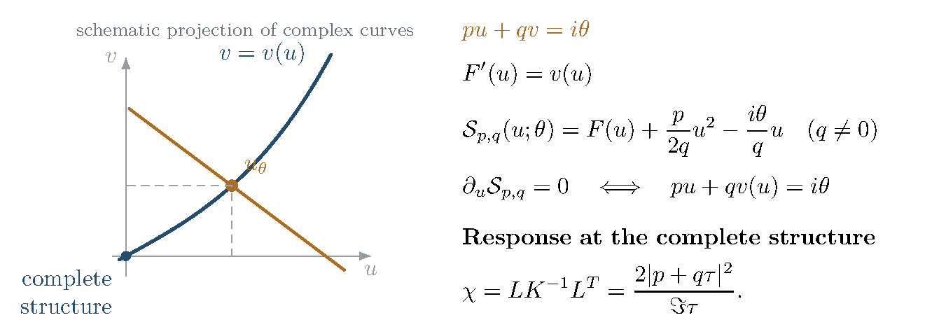
This is an exact identity of analytic germs, so it compares all orders of the two classical expansions. For $q=0$, exchange the oriented basis to $(\mu',\lambda')=(\lambda,-\mu)$; the new slope has $q'=-p\ne0$. The real angle optimization itself needs no such basis change. Primitive $q=0$ slopes have $p=\pm1$ and do not occur in a long-slope sequence in a fixed basis. Figure 6 records the local intersection condition and the response at the complete structure.

16.5 The Neumann–Zagier coefficients through sixth order

Series inversion of (16.2) gives $$u_\theta=\frac{i\theta}{A} +\frac{iqc_3\theta^3}{A^4} +i\theta^5\left(\frac{3q^2c_3^2}{A^7} -\frac{qc_5}{A^6}\right)+\cdots.$$(16.14) Substitution in the action, or integration of the envelope derivative, gives $$\mathcal S^*(\theta)=\frac{\theta^2}{2qA} +\frac{c_3\theta^4}{4A^4} +\frac{\theta^6}{6} \left(\frac{3qc_3^2}{A^7}-\frac{c_5}{A^6}\right)+\cdots.$$(16.15) Taking half its imaginary part yields the volume loss $$\begin{aligned} V_0-V_{p,q}(\theta) ={}&\frac{B\theta^2}{4|A|^2} -\frac{\theta^4}{8}\Im\frac{c_3}{A^4}\\ &-\frac{\theta^6}{12} \Im\left(\frac{3qc_3^2}{A^7}-\frac{c_5}{A^6}\right) +O(|A|^{-8}). \end{aligned}$$ Here the displayed remainder is a long-slope estimate for bounded $\theta$, on the common holonomy neighborhood constructed above. The uniform analytic inverse expands in $i\theta/A$ with coefficients analytic in the bounded parameter $q/A$; the next volume terms are therefore $O(|A|^{-8})$. Since $q/A$ is bounded, the three displayed terms have orders $|A|^{-2},|A|^{-4},|A|^{-6}$. For a fixed slope and $\theta\to0$, the corresponding Taylor remainder is $O(\theta^8)$.

For the smooth hyperbolic filling $M_{p/q}$ this becomes $$\begin{aligned} \boxed{\begin{aligned} V_0-\mathop{\mathrm{Vol}}(M_{p/q}) ={}&\frac{\pi^2B}{|A|^2} -2\pi^4\Im\frac{c_3}{A^4}\\ &-\frac{16\pi^6}{3} \Im\left(\frac{3qc_3^2}{A^7}-\frac{c_5}{A^6}\right) +O(|A|^{-8}). \end{aligned}} \end{aligned}$$ These are the Neumann–Zagier coefficients, with the multiplier normalization fixed explicitly [36, Section 6]. In particular the leading loss is $\pi^2/Q(p,q)$, and the quartic term detects the first nonlinear deformation coefficient $c_3$.

16.6 Computing the quartic coefficient from angle-volume derivatives

The comparison supplies a more detailed computational identity. Keep $K,L,\chi$ as above, and write $$T_3=D^3\mathscr V(0),\qquad T_4=D^4\mathscr V(0),\qquad e=\frac{K^{-1}L^T}{\chi},\qquad R=K^{-1}-\frac{K^{-1}L^TLK^{-1}}{\chi}.$$ Let $t=T_3(e,e,\cdot)$ be the resulting column covector. Solving the constrained stationary equation to second order gives $$x_\theta=\theta e+\frac{\theta^2}{2}Rt+O(\theta^3).$$ Indeed $Le=1$, $LR=0$, and $RK$ is the identity on $\ker L$. Inserting this expression into the Taylor expansion of $\mathscr V$ gives $$\begin{aligned} V_{p,q}(\theta)={}&V_0-\frac{\theta^2}{2\chi} +\frac{\theta^3}{6}T_3[e,e,e]\\ &+\frac{\theta^4}{24} \left(T_4[e,e,e,e]+3t^TRt\right)+O(\theta^5). \end{aligned}$$ The cross term with the unknown cubic displacement vanishes because that displacement is in $\ker L$ and $Ke=L^T/\chi$. The remaining quadratic-displacement terms combine to $t^TRt/8$. Evenness of the geometric branch then removes the odd coefficients and improves the remainder to $O(\theta^6)$. Comparison with (16.16) yields $$\boxed{T_3[e,e,e]=0,\qquad T_4[e,e,e,e]+3t^TRt =3\Im\frac{c_3}{(p+q\tau)^4}.}$$(16.19) Thus $c_3$ can be accessed from derivatives of the angle-volume functional by varying the slope. The correction $3t^TRt$ accounts for readjustment of all other angles. Keeping only the raw fourth derivative would miss that response.

16.7 The closed quantum-volume statement and its local consequence

A precise closed-manifold analogue is the Chen–Yang volume conjecture. At the specified root $\zeta_r=e^{2\pi i/r}$, with $r$ odd, its absolute-growth statements are $$\frac{4\pi}{r}\log|\mathrm{RT}_r(N;\zeta_r)|\longrightarrow\mathop{\mathrm{Vol}}(N), \qquad \frac{2\pi}{r}\log\mathrm{TV}_r(N;\zeta_r)\longrightarrow\mathop{\mathrm{Vol}}(N).$$(16.20) The root and normalization matter; these are the Chen–Yang versions for hyperbolic manifolds [38]. We use absolute growth to avoid mixing the different Chern–Simons sign conventions in the literature.

For a boundary state whose geometric semiclassical phase satisfies $$\Phi(u)=\Phi_0+\frac12F(u),\qquad \Im\Phi_0=V_0,$$ the filling phase is $$\mathcal T_\theta(u)=\Phi_0+\frac12\mathcal S_{p,q}(u;\theta).$$(16.21) Possible real framing constants do not alter its imaginary part. With $\hbar_r=4\pi i/r$, Proposition 16.1 immediately gives $$\left|e^{\mathcal T_\theta(u_\theta)/\hbar_r}\right| =\exp\left(\frac{r}{4\pi}V_{p,q}(\theta)\right).$$(16.22) In particular, the deformation of the geometric exponential is $$\log\left|\frac{e^{\mathcal T_\theta(u_\theta)/\hbar_r}} {e^{\Phi_0/\hbar_r}}\right| =-\frac{r}{4\pi}\bigl(V_0-V_{p,q}(\theta)\bigr).$$(16.23) Every classical coefficient in (16.16) therefore appears with precisely the required quantum exponential coefficient. At $\theta=2\pi$, Yoshida’s complex-volume formula has this normalization; see the unnumbered filling formula and the potential normalization (5.9) on [40, p. 456]. Quadratic and linear filling kernels also appear explicitly in [39, equations (12)–(14)]; their boundary coordinates and level conventions must be converted before numerical coefficients are compared.

For a general knot this proposition identifies the needed analytic input; it does not establish that input from a complete-point Kashaev asymptotic alone. A value at $u=0$ does not provide a uniform boundary-state expansion near $0$, and a local critical point does not by itself specify its coefficient in the global surgery sum. The regular tetrahedral Airy formula in Section 15 concerns a different integral and does not supply that missing manifold-level information.

16.8 The Gaussian factor and the torsion surgery formula

The derivative of the filling map is $$D_*:=p+qv'(u_\theta),\qquad \frac{\mathop{}\!\mathrm du_\theta}{\mathop{}\!\mathrm d\theta}=\frac{i}{D_*},\qquad \mathcal S_{uu}(u_\theta;\theta)=\frac{D_*}{q}.$$(16.24) Thus the same quantity controls the classical susceptibility and the Gaussian surgery integral. With the usual square-root normalization of the boundary Fourier kernel, its contribution has dependence $D_*^{-1/2}$, up to the common normalization and phase choices. A full amplitude also contains the boundary-state torsion and a solid-torus factor.

More precisely, suppose $\theta=2\pi$ gives a smooth hyperbolic filled manifold and the representation is its holonomy. Assume its adjoint representation is acyclic and its restriction to the compact core is regular for both $\mu$ and $p\mu+q\lambda$: the peripheral invariant vector paired with either curve supplies a basis of the one-dimensional twisted $H_1$, with the compatible boundary basis in $H_2$. In the local holonomy chart this requires $D_*\ne0$; the core is loxodromic, so $\sinh(w/2)\ne0$. The change-of-peripheral-curve and surgery formulas for adjoint Reidemeister torsion then give $$\begin{aligned} \operatorname{Tor}_{p\mu+q\lambda}(M_u) &=\bigl(p+qv'(u)\bigr)\operatorname{Tor}_\mu(M_u),\\ \operatorname{Tor}(M_{p/q}) &=\frac{\operatorname{Tor}_{p\mu+q\lambda}(M_u)} {4\sinh^2(w/2)},\qquad w=\rho u+\sigma v. \end{aligned}$$ These are understood up to the standard torsion signs and consistent choices of square root. They are the identities used in [40, equations (5.16) and (5.23)]. For the general regularity and change-of-curve statements, see [129, Propositions 5.13–5.14]; its Proposition 4.23(b), specialized to the adjoint representation $(k_1,k_2)=(2,0)$, gives the surgery factor up to the torsion sign. Consequently the expected full geometric amplitude is proportional to $$\boxed{ \frac{2\sinh(w/2)} {\sqrt{\bigl(p+qv'(u)\bigr)\operatorname{Tor}_\mu(M_u)}} =\frac{1}{\sqrt{\operatorname{Tor}(M_{p/q})}}.}$$(16.26) The identity shows what must accompany the boundary Hessian. Matching the Gaussian factor alone would leave out both the cusp torsion and the solid-torus amplitude. This one-loop comparison uses more information than the classical volume exponent. The closed-manifold torsion in this formula is evaluated at smooth filling; it is not being assigned to a generic cone holonomy. At the cusp endpoint $\theta=0$ the solid-torus factor vanishes, so a uniform quantum statement including that endpoint requires a separate normalization and analysis. The compact parameter interval in Proposition 16.2 is subject to its nonvanishing-amplitude hypothesis.

16.9 A figure-eight benchmark and the scope of the conclusion

For the figure-eight knot complement, in the standard peripheral basis Neumann–Zagier compute [36, equation (68)] $$v(u)=2\sqrt3\,i\left(u+\frac{u^3}{3} +\frac{23u^5}{180}+O(u^7)\right).$$(16.27) Thus $\tau=2\sqrt3\,i$, $c_3=2i/\sqrt3$, and $c_5=23i/(30\sqrt3)$. The first two volume-loss terms are $$\begin{aligned} V_0-\mathop{\mathrm{Vol}}(M_{p/q})={}&\frac{2\sqrt3\,\pi^2}{p^2+12q^2}\\ &-\frac{4\pi^4}{\sqrt3} \frac{p^4-72p^2q^2+144q^4}{(p^2+12q^2)^4} +O\bigl((p^2+q^2)^{-3}\bigr). \end{aligned}$$ This agrees directly with the expansion following equation (68) in [36]. The angle-Hessian response is correspondingly $$\chi=\frac{p^2+12q^2}{\sqrt3}.$$

An independent calculation starts with the two regular ideal tetrahedra and their Lobachevsky volume. In the Neumann–Zagier presentation their shapes $z_1,z_2$ satisfy $$z_1z_2(z_1-1)(z_2-1)=1,\qquad u=\log\bigl(z_2(1-z_1)\bigr),\qquad v=2\log\bigl(z_1(1-z_1)\bigr).$$ Eliminating the shapes from these equations gives the local peripheral relation $$\cosh(v/2)=1+\cosh u-\cosh(2u).$$ Equivalently, with the eigenvalue variables $m=e^{u/2}$ and $l=-e^{v/2}$, it is $l+l^{-1}=m^4-m^2-2-m^{-2}+m^{-4}$, the nonabelian figure-eight $A$-polynomial relation in this choice of signs. The sign in $l$ is essential: its complete value is $-1$ whereas $v(0)=0$. The equation and the chosen tangent $v'(0)=2\sqrt3\,i$ recover the cubic and quintic coefficients above. This is a local branch calculation, not a classification of the global curve or of fillings.

Use $\alpha_i=\arg z_i$, $\beta_i=-\arg(1-z_i)$, and $\gamma_i=\pi-\alpha_i-\beta_i$. Choose the independent variations $\xi=(\delta\alpha_1,\delta\beta_1,\delta\alpha_2)$. The edge equation then makes the six angle variations $$E\xi=(\xi_1,\xi_2,-\xi_1-\xi_2, \xi_3,\xi_1-\xi_2+\xi_3,-\xi_1+\xi_2-2\xi_3).$$ At the complete structure all six angles are $\pi/3$. Since $\Lambda''(\alpha)=-\cot\alpha$, direct differentiation gives $$K=\frac1{\sqrt3} \begin{pmatrix}4&-1&3\\-1&4&-3\\3&-3&6\end{pmatrix},\qquad P=\begin{pmatrix}0&-1&1\\2&-2&0\end{pmatrix},\qquad P K^{-1}P^T=\frac1{\sqrt3} \begin{pmatrix}1&0\\0&12\end{pmatrix}.$$(16.29) This recovers the cusp shape directly from the optimizer. Put $D_0=p^2+12q^2$. The unit angular-response vector is $$e=\frac{(6q-p,-6q-p,p-6q)^T}{2D_0}.$$ Using $$\Lambda'''(\pi/3)=\frac43,\qquad \Lambda''''(\pi/3)=-\frac8{3\sqrt3},$$ the six entries of $Ee$ occur in opposite pairs, so $T_3[e,e,e]=0$. Direct contraction of the fourth derivative and the constrained inverse-Hessian correction gives $$T_4[e,e,e,e]+3t^TRt =\frac{2\sqrt3\,(p^4-72p^2q^2+144q^4)}{D_0^4}.$$(16.30) Multiplying by $\theta^4/24$ and setting $\theta=2\pi$ gives the quartic filled-volume term in (16.28) with the opposite sign, as required for volume rather than volume loss. Thus the real optimization and the holomorphic series agree in a calculation made directly from the tetrahedral volume derivatives.

For this example there is also a theorem about the actual quantum invariants: Wong–Yang prove the leading RT asymptotic with relative error $O(r^{-1})$, and the RT/TV volume conjectures for every hyperbolic rational Dehn filling of the figure-eight knot [40, Theorems 1.1 and 1.2]. Their leading amplitude is the inverse square root of adjoint torsion, with their specified overall constant. Thus the local consistency calculation above is contained in a stronger result in that example. The present discussion reorganizes the comparison around volume optimization and its derivatives; it does not produce a new case of the quantum-volume conjecture.

For a general knot, the unconditional results here are the classical critical-value identity and its coefficient dictionary. The quantum conclusion for a specified local geometric contribution follows under the stated stationary-phase hypotheses. Passing to the full invariant requires control of its exact surgery representation and all competing contributions. One should first keep the filling slope fixed while taking $r\to\infty$, and then study the long-slope coefficients. A simultaneous limit in which the slope grows with $r$ requires uniform estimates not supplied by separate fixed-slope expansions.

The computational companion in experiments/quantum_surgery/README.md, with output at artifacts/quantum_surgery/result.json, checks finite formal series, canonical-coordinate identities, and the figure-eight angle-Hessian contractions in exact arithmetic. These fixtures check the displayed coefficient algebra. They do not compute a filled hyperbolic manifold or an exact quantum invariant, and do not establish convergence, a global integration cycle, or its noncancellation.

16.10 The symplectic pairing behind the calculation

The pairing in Neumann–Zagier is the structure behind the preceding formulas. It identifies the peripheral variables as conjugate coordinates, makes the geometric deformation locus Lagrangian, and fixes the canonical transformation for Dehn filling. We record the normalization explicitly, since interchanging meridian and longitude or using eigenvalue rather than multiplier logarithms changes the displayed signs or factors.