23 Simple multicurve coefficients of a twisted trace formula

23.1 Broken geodesics and the effect of reconnection

Colin de Verdière’s construction approximates loop space by broken geodesics and applies stationary phase to a complex heat parametrix [19]. For an equal time subdivision the finite-dimensional energy is $$E_N(x_0,\ldots,x_{N-1}) =N\sum_{i=0}^{N-1}d(x_i,x_{i+1})^2,\qquad x_N=x_0,$$ with consecutive points within the injectivity radius. The critical equations match incoming and outgoing velocities; the critical value for a constant-speed closed geodesic is $\ell_\gamma^2$. On a hyperbolic surface every closed geodesic, including a self-intersecting one, has positive transverse length Hessian. For a unit-speed parametrization and a periodic normal variation $f(s)N(s)$ this is $$\delta^2L_\gamma(f,f) =\int_0^{\ell_\gamma}\bigl((f')^2+f^2\bigr)\,\mathop{}\!\mathrm ds.$$ Consequently simplicity cannot be selected by retaining only positive Hessians in the ordinary loop space.

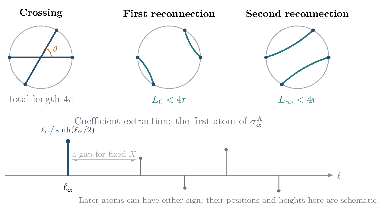
Reconnection enlarges that space. In a small embedded disk of radius $r$ about a transverse crossing of angle $\theta\in(0,\pi)$, the two original diameters have total length $4r$. The two noncrossing pairings have lengths $$\begin{aligned} L_0&=4\mathop{\mathrm{arsinh}}\bigl(\sinh r\sin(\theta/2)\bigr),\\ L_\infty&=4\mathop{\mathrm{arsinh}}\bigl(\sinh r\cos(\theta/2)\bigr). \end{aligned}$$ Both are strictly less than $4r$. In particular, $$4r-L_0=4r\bigl(1-\sin(\theta/2)\bigr)+O(r^3).$$ The descent is first order in the surgery radius. Tightening the resolved components to geodesics, and discarding contractible components, cannot increase total length. This is a change of connectivity, not a negative direction of the original Hessian. An unconstrained global minimization would select the empty cycle; we instead keep the different multicurves as algebraic observables.

23.2 The finite coefficient distributions

Let $\mathscr C(S)$ be the set of essential simple multicurves on the underlying marked surface. For $\rho:\pi_1(S)\to\mathrm{SU}(2)$ set $$T_C(\rho)=\prod_{\alpha\subset C}\mathop{\mathrm{tr}}\rho(\alpha), \qquad T_\varnothing=1.$$(23.2) The phrase “unnegated trace basis” refers to this sign convention, not to positivity of the function on $\mathrm{SU}(2)$. The functions $T_C$ are linearly independent on the unitary character variety and form a basis of the complex character ring after complexification; see Charles–Marché [20, Theorem 1.1]. The usual Kauffman convention uses $-\mathop{\mathrm{tr}}$ per component, so differs by a basis sign. The relation $$\mathop{\mathrm{tr}}A\,\mathop{\mathrm{tr}}B=\mathop{\mathrm{tr}}(AB)+\mathop{\mathrm{tr}}(AB^{-1})$$ resolves crossings. For every nontrivial closed curve $\gamma$ there is a unique finite expansion $$\mathop{\mathrm{tr}}\rho(\gamma)=\sum_{C\in\mathscr C(S)}a_C(\gamma)T_C(\rho), \qquad a_C(\gamma)\in\mathbb Z.$$(23.3) These integers depend only on topology, not on $X$.

Let $\Delta_\rho$ be the rank-two flat unitary bundle Laplacian, and write $\lambda_j(\rho)=1/4+r_j(\rho)^2$. For an even $\varphi\in C_c^\infty(\mathbb R)$ put $$h(r)=\int_\mathbb R\varphi(L)e^{irL}\,\mathop{}\!\mathrm dL,$$ and define $$\begin{aligned} \mathscr T^X_\varphi(\rho) &=\sum_j h(r_j(\rho)) -\frac{2\operatorname{Area}(X)}{4\pi} \int_\mathbb Rr h(r)\tanh(\pi r)\,\mathop{}\!\mathrm dr. \end{aligned}$$ With the two orientations grouped, the twisted Selberg formula is $$\mathscr T^X_\varphi(\rho) =\sum_{\delta\in\mathcal P_{\mathrm{un}}} \sum_{k\geq1} \frac{\ell_\delta}{\sinh(k\ell_\delta/2)} \varphi(k\ell_\delta)\mathop{\mathrm{tr}}\rho(\delta^k).$$(23.4) Here $\mathcal P_{\mathrm{un}}$ consists of unoriented primitive closed geodesics. Naud’s statement [21, Theorem 2.2] sums over oriented primitive conjugacy classes with denominator $2\sinh$; grouping inverses gives (23.4). The compact length support makes the geometric sum finite.

Local finiteness follows from the finiteness of the closed-geodesic length set below any bound. The identity term in the trace formula is a constant function of $\rho$, hence affects only the empty multicurve coefficient. The input is the labelled family $\rho\mapsto\operatorname{Spec}\Delta_\rho$ on the marked character variety. A scalar spectrum alone does not retain these coefficients.

23.3 Length triangularity and the first atom

For $m=1$ the first atom determines both the simple length and its normalization. Choose a fixed smooth cutoff $\chi$, equal to one near $\ell_\alpha$ and supported away from every other atom in a small neighborhood of $X$. Then $$\boxed{ \ell_X(\alpha) =\frac{\langle\sigma_\alpha^X,L\chi(L)\rangle} {\langle\sigma_\alpha^X,\chi(L)\rangle},\qquad \langle\sigma_\alpha^X,\chi\rangle =\frac{\ell_\alpha}{\sinh(\ell_\alpha/2)}. }$$(23.7) This is an exact localized identity, with no limiting interchange. Figure 7 relates the local reconnections to this separate first-atom statement for a simple support.

23.4 An exponential coefficient bound from bracelet positivity

The passage from compactly supported tests to heat kernels needs a growth estimate. A direct crossing count gives an exponential in $\ell_\gamma^2$ and only a small-time conclusion. Bracelet positivity gives a stronger estimate.

At skein parameter $+1$, Dylan Thurston proves that every diagram has a sign-coherent expansion in the bracelet basis [22, Theorem 2]. A bracelet supported on a simple curve $\beta$ with winding $n$ is the Chebyshev element $P_n(z_\beta)$ [22, Proposition 4.4]. Distinct bracelet support curves are disjoint; their windings are included in the length $\ell_X(D)=\sum_i n_i\ell_X(\beta_i)$. The canonical twisted Fuchsian evaluation associated to $X$ is positive on bracelet basis elements: $$B_D(X)=\prod_i2\cosh\bigl(n_i\ell_X(\beta_i)/2\bigr)>0.$$ For a one-component diagram representing $\gamma$, its evaluation has absolute value $2\cosh(\ell_X(\gamma)/2)$. Sign coherence therefore gives $$\sum_D |b_D(\gamma)| B_D(X) =2\cosh\bigl(\ell_X(\gamma)/2\bigr).$$(23.8) A spin structure identifies the $+1$ and $-1$ skein algebras by signs on diagrams. Changing to (23.2) also changes only basis signs. On a simple generator this replaces $z_\beta$ by $\epsilon_\beta T_\beta$, with $\epsilon_\beta\in\{1,-1\}$; the identity $P_n(\epsilon x)=\epsilon^nP_n(x)$ shows that the bracelet-to-multicurve coefficient magnitudes are unchanged. All the absolute estimates below are consequently valid in our unnegated trace basis. The positive Fuchsian evaluation is an auxiliary algebraic estimate; the Laplacians defining $\sigma_C^X$ still use unitary twists.

For a single simple $\alpha$ one can use $$K_{\alpha,X} =\sup_{\substack{n\geq1\\n\text{ odd}}} \frac{n}{2\cosh(n\ell_\alpha/2)} \leq\frac{2}{e\ell_\alpha}.$$ The estimates are uniform for a fixed target $C$ on compact subsets of Teichmüller space. Related positivity and Chebyshev estimates for analytic lamination expansions on punctured planar surfaces appear in Basok–Chelkak [23, Section 4.4, Theorems 4.7 and 4.9]. Their full analytic expansion theorem is not needed here.

23.5 Convergent heat and Laplace transforms

Define $$\begin{aligned} G_C^X(t)&=\int_0^\infty e^{-L^2/(4t)}\,\mathop{}\!\mathrm d\sigma_C^X(L), &H_C^X(t)&=\frac{e^{-t/4}}{\sqrt{4\pi t}}G_C^X(t), \\ D_C^X(s)&=\int_0^\infty e^{-sL}\,\mathop{}\!\mathrm d\sigma_C^X(L). && \end{aligned}$$ By (23.11), $G_C$ and $H_C$ are absolutely convergent for every $t>0$, and holomorphic for $\Re t>0$ with the principal square root. The Laplace transform is absolutely convergent and holomorphic for $\Re s>1$. Differentiation in these variables is permitted locally uniformly in the stated domains.

There is also a convergent expansion of the whole heat trace. For a finite character polynomial set $$\|f\|_2=\sum_C|[T_C]f|\,2^{\#C},\qquad c_X=\frac{\log(1+\sqrt2)}{\operatorname{sys}(X)}.$$ The subscript $2$ denotes the trace bound $|\mathop{\mathrm{tr}}\rho(\alpha)|\leq2$; this is a weighted coefficient norm, not an $L^2$ norm. The Chebyshev recurrence gives $$\sum_r|[x^r]P_n(x)|2^r\leq2(1+\sqrt2)^n.$$ A bracelet has at most $3g-3$ distinct support curves, so $\|B_D\|_2\leq2^{3g-3}e^{c_X\ell_X(D)}$. In (23.8) the nonzero coefficients are integers, and $B_D(X)\geq e^{\ell_X(D)/2}$. Hence $\ell_X(D)\leq\ell_X(\gamma)+2\log2$ for every occurring $D$, and $\sum_D|b_D|\leq2e^{\ell_X(\gamma)/2}$. Therefore $$\|\mathop{\mathrm{tr}}_\gamma\|_2\leq C_X e^{(1/2+c_X)\ell_X(\gamma)},\qquad C_X=2^{3g-2}e^{2c_X\log2}.$$(23.14) Gaussian decay dominates this exponential bound and the orbit count. It follows that $$\boxed{ \operatorname{Tr}e^{-t\Delta_\rho}-2I_X(t) =\sum_{C\in\mathscr C(S)}H_C^X(t)T_C(\rho),\qquad t>0, }$$(23.15) where $$I_X(t)=\frac{\operatorname{Area}(X)}{4\pi} \int_\mathbb Rr\tanh(\pi r)e^{-t(r^2+1/4)}\,\mathop{}\!\mathrm dr, \qquad \sum_C|H_C^X(t)|2^{\#C}<\infty.$$ The series is uniform on the unitary character variety and locally uniform for $\Re t>0$. It is obtained by taking the limit of the finite length-cutoff expansions; the preceding absolute estimate justifies the rearrangement. For a compact set of such $t$, $\Re(1/t)$ has a positive lower bound, so the same Gaussian majorant proves local uniformity and termwise holomorphy. On the spectral side, smooth cutoffs of the Gaussian converge in the Schwartz topology on the real spectral axis and at the finitely many imaginary spectral parameters; the compact-surface Weyl bound justifies passing to the heat trace for each unitary twist.

This construction does not assert uniqueness among arbitrary infinite expansions of a continuous function. For example, $\|\mathop{\mathrm{tr}}\rho(\alpha^{2n+1})\|_\infty\leq2$, while its $T_\alpha$ coefficient is $(-1)^n(2n+1)$. Coefficient extraction is therefore not bounded for the uniform norm on unitary characters. Our coefficients are fixed by the finite spectral tests first; the estimates then justify their heat transform.

After removing the explicit $e^{-t/4}$ factor, the correction to the single-geodesic term is exponentially small, rather than a new power series in $t$. Thus the constant-curvature heat coefficient has an exact isolated-orbit prefactor, followed by contributions at larger length actions. For $m\alpha$ replace the action by $(m\ell_\alpha)^2/(4t)$ and the mass by $\ell_\alpha/\sinh(m\ell_\alpha/2)$.

23.6 All iterates of a simple curve

Write $\sigma_C^{X,[\delta]}$ for the contribution of one primitive unoriented class $\delta$ and all of its iterates. The polynomial identity $$P_k(x)=\sum_{j=0}^{\lfloor k/2\rfloor} (-1)^j\frac{k(k-j-1)!}{j!(k-2j)!}x^{k-2j},\qquad k\geq1,$$(23.19) follows from the recurrence. If $\alpha$ is simple, the coefficient of $m\alpha$ vanishes unless $k=m+2j$, and for $m\geq1$ is $$b_{m+2j,m}=(-1)^j \frac{(m+2j)(m+j-1)!}{j!\,m!}.$$(23.20) In particular, with $\ell=\ell_\alpha$, $$\boxed{ \sigma_\alpha^{X,[\alpha]} =\ell\sum_{j\geq0} \frac{(-1)^j(2j+1)}{\sinh((2j+1)\ell/2)} \delta_{(2j+1)\ell}. }$$(23.21) The first masses have multipliers $1,-3,5,-7,\ldots$ at $\ell,3\ell,5\ell,7\ell,\ldots$. For $2\alpha$ the multipliers are $1,-4,9,-16,\ldots$ at $2\ell,4\ell,6\ell,8\ell,\ldots$. These are explicit later atoms, not changes to the first-atom mass.

For $m\geq1$ the coefficient generating function is $$B_m(q):=\sum_{k\geq1}b_{k,m}q^k =\frac{q^m(1-q^2)}{(1+q^2)^{m+1}}.$$(23.22) Indeed, $\sum_{k\geq1}P_k(x)q^k=(xq-2q^2)/(1-xq+q^2)$, and extracting $x^m$ gives this formula. Expanding the hyperbolic denominator yields, for $\Re s>-1/2$, $$\begin{aligned} D_{m\alpha}^{X,[\alpha]}(s) &=2\ell\sum_{n\geq0}B_m(q_n), &q_n&=e^{-(s+n+1/2)\ell},\\ &=2^{1-m}\ell\sum_{n\geq0} \mathop{\mathrm{sech}}^m(u_n)\tanh(u_n), &u_n&=(s+n+1/2)\ell. \end{aligned}$$ This larger convergence domain concerns the one fixed primitive family; the proved half-plane for the full $D_C$ is $\Re s>1$.

The heat contribution of the same family is $$\begin{aligned} H_\alpha^{X,[\alpha]}(t) ={}&\frac{e^{-t/4}}{\sqrt{4\pi t}} \frac{\ell e^{-\ell^2/(4t)}}{\sinh(\ell/2)}\\ &\mathrel{}\times\left[ 1-3\frac{\sinh(\ell/2)}{\sinh(3\ell/2)}e^{-2\ell^2/t} +5\frac{\sinh(\ell/2)}{\sinh(5\ell/2)}e^{-6\ell^2/t} -\cdots\right]. \end{aligned}$$ Other primitive classes may supply corrections before these particular iterate actions. Once $\ell_\alpha$ is recovered, subtracting the $j\geq1$ terms of (23.21) removes exactly the nonprimitive powers of the simple curve $\alpha$; it leaves powers of nonsimple curves that resolve with an $\alpha$ coefficient.

23.7 A figure-eight family and an exact cancellation

Take an embedded geodesic pair of pants with three distinct essential cuffs $a,b,c$, and $c=(ab)^{-1}$. Set $$x=T_a,\qquad y=T_b,\qquad z=T_c,\qquad \gamma=a^{-1}b, \qquad T_\gamma=xy-z.$$ These are functions of arbitrary unitary holonomy. The minus sign therefore differs from the positive hyperbolic length convention in (18.1). Powers are given exactly by $T_{\gamma^k}=P_k(xy-z)$. For example, $$\begin{aligned} T_\gamma&=xy-z,\\ T_{\gamma^2}&=x^2y^2-2xyz+z^2-2,\\ T_{\gamma^3}&=x^3y^3-3x^2y^2z+3xyz^2-z^3-3xy+3z. \end{aligned}$$ Only multicurves $C=ra+rb+mc$ occur. Put $d=r+m\geq1$. Their coefficients vanish unless $k=d+2j$, and in that case $$\boxed{ a_{ra+rb+mc}(\gamma^k) =(-1)^{j+m}\frac{k(k-j-1)!}{j!\,r!\,m!} =(-1)^m\binom{r+m}{r}b_{k,r+m}. }$$(23.25) This follows by substituting $xy-z$ into (23.19) and expanding the relevant monomial. Consequently $$\sum_{k\geq1}a_{ra+rb+mc}(\gamma^k)q^k =(-1)^m\binom{r+m}{r} \frac{q^{r+m}(1-q^2)}{(1+q^2)^{r+m+1}}.$$

For $r+m=1$ the two target coefficients are opposite for every iterate. If $L=\ell_\gamma$, then $$\boxed{ \sigma_{a+b}^{X,[\gamma]} =-\sigma_c^{X,[\gamma]} =L\sum_{j\geq0} \frac{(-1)^j(2j+1)}{\sinh((2j+1)L/2)} \delta_{(2j+1)L}. }$$(23.26) Thus $\sigma_c^X+\sigma_{a+b}^X$ cancels the entire chosen figure-eight family, including all its powers. This does not assert that the full sum vanishes: other primitive classes contribute to both coefficients. It gives an exact family-by-family cancellation which is preserved by either transform in (23.12)–(23.13).

The distinct-cuff assumption makes the monomials above distinct multicurve basis elements. If cuff images coincide, as in some one-holed-torus configurations of Section 18, the corresponding variables must first be identified and equal basis terms collected; the displayed coefficient indexing cannot be carried over unchanged.

23.8 Metric variation and the twist derivative

For a fixed topological $C$, the map $X\mapsto\sigma_C^X$ is smooth as a distribution-valued map. After applying any compactly supported test function, it is locally a finite sum of smooth length functions. It is not asserted to be real analytic for arbitrary smooth test functions.

For an orbital label $(\delta,k)$ write $$L=k\ell_\delta,\qquad w=\ell_\delta\operatorname{csch}(L/2).$$ For a tangent vector $v$ to Teichmüller space one has $$D_v\sigma_C^X =\sum_{\delta,k}a_C(\delta^k) \left[(D_vw)\delta_L-w(D_vL)\delta'_L\right],$$(23.27) where $\langle\delta'_L,\varphi\rangle=-\varphi'(L)$ and $$D_vL=kD_v\ell_\delta,\qquad D_vw=\operatorname{csch}(L/2) \left(1-\frac L2\coth\frac L2\right)D_v\ell_\delta.$$ The coefficients $a_C$ are constant under metric variation. This formula describes movement of the atoms as well as variation of their masses; omitting the $\delta'_L$ term would lose the length variation itself.

For a twist of displacement $\tau_\beta$ about a simple geodesic $\beta$, Wolpert’s cosine formula gives $$\frac{\partial\ell_\delta}{\partial\tau_\beta} =\sum_{p\in\delta\cap\beta}\cos\theta_p,$$(23.28) with the consistent right-twist angle convention and intersections counted with multiplicity [24]. Substitution in (23.27) gives an exact variation formula for every coefficient distribution. For a simple $\alpha$, one can equivalently differentiate the localized ratio (23.7); it recovers (23.28) from two spectral coefficient moments, without an infinite limit. The first-variation argument also applies when $\delta$ is immersed: cut it at its crossings with $\beta$. Interior variations of the geodesic arcs cancel by stationarity; the relative tangential displacement at each paired endpoint contributes the projection $\cos\theta_p$. Summing over the passages through the cut gives the formula with precisely the stated multiplicities. If $\delta$ is a power of $\beta$, its twist derivative is zero and the sum is interpreted as empty.

The compact-set gap in Proposition 23.3 also permits differentiating the leading heat asymptotic locally. The leading logarithmic response is $$D_v\log H_\alpha^X(t) =\left[-\frac{\ell_\alpha}{2t} +\frac1{\ell_\alpha} -\frac12\coth\frac{\ell_\alpha}{2}\right] D_v\ell_\alpha +O\bigl(t^{-1}e^{-c/t}\bigr)$$(23.29) for some local $c>0$. To justify the differentiated tail, metric length derivatives on a compact parameter neighborhood are bounded by constants times the length, while (23.9) is locally uniform. Gaussian decay absorbs the additional polynomial factors.

23.9 The logarithmic product and primitive extraction

A useful connection to the Selberg product keeps the orientation normalization explicit. Define, for $\Re v>1$, $$\mathcal Z_\rho^X(v) =\prod_{\delta\in\mathcal P_{\mathrm{un}}}\prod_{n\geq0} \det\left(I-e^{-(v+n)\ell_\delta}\rho(\delta)\right).$$(23.30) This definition uses unoriented primitives; a product over both oriented conjugacy classes squares it. Expanding the logarithm gives $$2\left.\frac{\partial}{\partial v} \log\mathcal Z_\rho^X(v)\right|_{v=s+1/2} =\sum_{\delta,k} \frac{\ell_\delta e^{-sk\ell_\delta}} {\sinh(k\ell_\delta/2)}\mathop{\mathrm{tr}}\rho(\delta^k).$$(23.31) With coefficients defined by finite length cutoffs, the $T_C$ coefficient on the right is $D_C^X(s)$ for $\Re s>1$. The coefficient estimate proves this assertion; it is not an appeal to continuity of coefficient extraction in the uniform norm. No meromorphic continuation of the individual $D_C$ is established by this calculation.

Removing all iterates by a global Chebyshev substitution is not legitimate in the rank-two character ring. If $x=\mathop{\mathrm{tr}}A$, $y=\mathop{\mathrm{tr}}B$, $u=\mathop{\mathrm{tr}}(AB)$, and $v=\mathop{\mathrm{tr}}(AB^{-1})$, then $u+v=xy$, but $$P_2(u)+P_2(v)-P_2(x)P_2(y) =2\bigl(\mathop{\mathrm{tr}}[A,B]-2\bigr),$$(23.32) which is generally nonzero. Thus sending every trace to its Chebyshev polynomial does not define a multiplicative operation on this character ring.

There is an exact repair if extra twisting data are supplied. For the original $\mathrm{SU}(2)$ representation $\rho$, work in the virtual representation ring generated by its symmetric powers. Let $\psi^k\rho$ denote its Adams operation, characterized by $\chi_{\psi^k\rho}(\gamma)=\chi_\rho(\gamma^k)$. For the standard rank-two representation, $$\psi^k\rho=\operatorname{Sym}^k\rho- \operatorname{Sym}^{k-2}\rho\quad(k\geq2), \qquad \psi^1\rho=\rho.$$ Trace formulas extend additively to virtual representations. All twists used here have inverse-invariant characters, so the unoriented normalization is preserved. Let $\Sigma_\rho$ denote the character-valued geometric measure on the right of (23.4), and set $$Q_\rho=\sinh(L/2)\Sigma_\rho,\qquad P_\rho=\sum_{\delta\in\mathcal P_{\mathrm{un}}} \ell_\delta\chi_\rho(\delta)\delta_{\ell_\delta}.$$ For $D_k\delta_L=\delta_{kL}$, $$Q_\rho=\sum_{k\geq1}D_kP_{\psi^k\rho},\qquad \boxed{P_\rho=\sum_{k\geq1}\mu(k)D_kQ_{\psi^k\rho}.}$$ These sums are locally finite, and the second identity follows from $\psi^j\psi^k=\psi^{jk}$ and divisor Möbius inversion. It requires spectra for higher symmetric-power twists, which are additional data beyond the original rank-two family. The explicit subtraction in (23.21) needs no such enlargement.

23.10 Scope and further questions

The construction now supplies signed coefficient distributions, an isolated first simple-curve atom, globally convergent heat transforms, a Laplace half-plane, explicit iterate families, a figure-eight cancellation, and metric derivatives. It has not produced a positive measure with the weights of simple-geodesic counting, nor a pointwise constant McShane series.

The scalar limitation is genuine: length-isospectral closed hyperbolic surfaces can have different simple length spectra [25]. The labelled holonomy family retains the information used by (23.7).

For a counting comparison, let $d=6g-6$ and normalize Thurston measure by the integral multicurve lattice. If $$B(X)=\mu_{\mathrm{Th}}\{\lambda:\ell_X(\lambda)\leq1\},$$ ordinary lattice counting gives $\#\{C\in\mathcal{ML}_{\mathbb Z}:\ell_X(C)\leq R\}\sim B(X)R^d$ [77, Proposition 3.1]. Its Laplace consequence is $$\sum_{C\in\mathcal{ML}_{\mathbb Z}}e^{-t\ell_X(C)} \sim\Gamma(d+1)B(X)t^{-d}\qquad(t\downarrow0).$$ This is a target for a measure comparison, not a consequence of the coefficient heat expansion. It counts all weighted multicurves; connected or fixed-orbit counts require additional information. The large-length limit here is also different from the minimum-selection limits in (23.18).

Two concrete further problems are to continue $D_C(s)$ beyond its proved half-plane, with control of the coefficient operation, and to find combinations of coefficients whose cancellations organize globally over pants. Formula (23.26) provides an exact local model for the second problem. An identity constant in $X$ would require an additional normalization or geometric partition; the existence of these transforms alone does not supply that constancy. Section 24 strengthens the lattice benchmark and gives explicit orbital gaps, uniform recovery estimates, and a conditional counting criterion.