10 A geometric introduction to the quantum constructions

10.1 Six labels: recoupling and tetrahedral weights

Let $V_j$ be the irreducible $\mathfrak{sl}_2$-representation of dimension $2j+1$, where $j$ is a nonnegative half-integer. Consider $$\operatorname{Hom}_{\mathfrak{sl}_2}(V_d,V_a\otimes V_b\otimes V_c).$$ There are two natural bases. One first decomposes $V_a\otimes V_b$ and records an intermediate representation $V_s$; the other first decomposes $V_b\otimes V_c$ and records $V_t$. Thus $$B_s^{(ab)c}=\sum_t F_{st}^{abc;d}B_t^{a(bc)}.$$(10.1) The coefficients depend on six labels $a,b,c,d,s,t$. With conventional dimension and sign factors, they are the $6j$-symbols. The four admissible triples $$(a,b,s),\quad(s,c,d),\quad(b,c,t),\quad(a,t,d)$$ can be assigned to the four faces of a tetrahedron. At this point the tetrahedron is a way to organize the labels. Its interpretation as a metric tetrahedron requires an additional asymptotic statement.

A quantum group deforms this tensor-product calculus. For $U_{q_{\mathrm{alg}}}(\mathfrak{sl}_2)$, ordinary integers and factorials in the explicit formulas are replaced by their quantum analogues, for example $$[n]_{q_{\mathrm{alg}}} =\frac{q_{\mathrm{alg}}^{n}-q_{\mathrm{alg}}^{-n}} {q_{\mathrm{alg}}-q_{\mathrm{alg}}^{-1}},\qquad [n]_{q_{\mathrm{alg}}}\longrightarrow n\quad(q_{\mathrm{alg}}\to1).$$(10.2) The full definition also specifies tensor products and braidings; it is not merely a rule for replacing integers. At the usual compact root $q_{\mathrm{alg}}=e^{\pi i/r}$, the finite fusion theory retains the labels $0,\frac12,\ldots,\frac{r-2}{2}$. A triple must satisfy the triangle inequalities, integral total spin, and $a+b+c\le r-2$. Taylor–Woodward give the representation-theoretic definition and these conventions explicitly [26].

Associating four tensor factors in the five possible ways gives the pentagon identity. In tetrahedral language it supplies the identity for replacing two tetrahedra by three in a triangulated ball. Together with orthogonality and normalization identities, this makes state sums independent of the triangulation. Schematically, a Turaev–Viro sum for a closed triangulated manifold has the form $$Z_r(M)=C_r(T)\sum_{\text{admissible edge labels }\mathbf j} \prod_{e\in E(T)}d_{j_e}\, \prod_{\Delta\in T}\{6j\}_{\Delta,\mathbf j}.$$(10.3) Here $T$ is a triangulation, $d_j$ is a quantum dimension, and $C_r(T)$ is the prescribed normalization. This displayed formula explains the structure; the exact weights are part of the definition of the chosen theory [38, Sections 2.2–2.3]. A state in this sum is an admissible assignment of labels. The sum is over such assignments; a description as an integral over hyperbolic metrics, with a particular geometric measure, would be a further result.

10.2 The invariants and their volume limits

The main objects used below can be distinguished by their inputs and outputs.

The first four objects are topological invariants with their prescribed normalizations. The last two supply analytic kernels and functions that enter the comparisons in this monograph. In particular, a local $6j$-weight is not already a three-manifold invariant.

The knot construction begins with a braid whose closure is the knot. A crossing acts by a braiding matrix on the tensor product of the strand representations; the Yang–Baxter equation gives the braid relation. A quantum trace, adjusted to the representation theory, closes the strands, and the prescribed normalization handles the moves that change the braid presentation [29, Section 2].

For the colored Jones polynomial, the color $N$ denotes the $N$-dimensional representation at generic parameter. We use the reduced normalization $J_N(\text{unknot};q_J)=1$, and specialize only after forming that polynomial. Murakami–Murakami identify this specialization with Kashaev’s invariant [82]. For a hyperbolic knot, the volume conjecture is $$\lim_{N\to\infty}\frac{2\pi}{N} \log|J_N(K;e^{2\pi i/N})|=\mathop{\mathrm{Vol}}(S^3\setminus K).$$(10.4) The right side is the ordinary three-dimensional hyperbolic volume, not a volume of moduli space. The assertion concerns a sequence in which both the color and the root change.

The closed-manifold version used in Section 16 is the Chen–Yang asymptotic at their root $\zeta_r=e^{2\pi i/r}$, with $r$ odd: $$\frac{4\pi}{r}\log|\mathrm{RT}_r(M;\zeta_r)|\longrightarrow\mathop{\mathrm{Vol}}(M), \qquad \frac{2\pi}{r}\log\mathrm{TV}_r(M;\zeta_r)\longrightarrow\mathop{\mathrm{Vol}}(M).$$(10.5) These statements are conjectural in general, with theorems for specified families; the hyperbolic fillings of the figure-eight used later are covered by Wong–Yang [40]. The doubling relation between matching RT and TV theories explains the factor two between their leading logarithms. Exact identities require consistent choices: generally $\mathrm{TV}_{\mathcal C}$ is the RT invariant of the categorical center, and the familiar modulus-square formula holds in the matching unitary modular setting [27]. One should not equate differently normalized $\mathrm{SU}(2)$ and $\mathrm{SO}(3)$ versions without conversion.

There are two root-of-unity subtleties. First, authors use parameters differing by a square: in a common convention $q_J=q_{\mathrm{alg}}^2$. Within Chen–Yang’s conventions, the volume root $e^{2\pi i/r}$ differs from the standard compact root $e^{\pi i/r}$; the latter belongs to a different asymptotic problem [38]. Second, even where the numerical roots agree after changing notation, the colors may not belong to the same theory. At $q_{\mathrm{alg}}=e^{\pi i/N}$, the $N$-dimensional color has $[N]_{q_{\mathrm{alg}}}=0$ and lies outside the retained simple labels of the level-$N-2$ compact fusion theory. Reducing $J_N$ first and then specializing is essential. Thus the Kashaev limit should not be read as an allowed fixed-color observable in that finite unitary theory.

10.3 A complete example: the figure-eight knot

For the figure-eight knot $4_1$, the root specialization is an especially simple positive sum: $$\boxed{\quad J_N(4_1;e^{2\pi i/N})=\sum_{k=0}^{N-1}P_{N,k},\qquad P_{N,k}=\prod_{j=1}^{k}4\sin^2\frac{\pi j}{N},\quad P_{N,0}=1. \quad}$$(10.6) Kashaev gives the product formula [28, eqs. (2.2), (2.5)]. The following elementary asymptotic proof is presented by Murakami and credited there to Ekholm [29, Section 3.2].

The ratio of consecutive products is $$\frac{P_{N,k}}{P_{N,k-1}}=4\sin^2\frac{\pi k}{N}.$$ It is less than one before $N/6$, greater than one between $N/6$ and $5N/6$, and less than one afterward. The global maximum is therefore attained at $m_N=\lfloor5N/6\rfloor$, allowing an adjacent tie. To compare with the initial value $1$, use the elementary identity $P_{N,N-1}=N^2$: evaluating $(z^N-1)/(z-1)=\prod_{j=1}^{N-1}(z-e^{2\pi i j/N})$ at $z=1$ and taking absolute squares proves it. Positivity now gives $$P_{N,m_N}\le J_N(4_1;e^{2\pi i/N})\le N P_{N,m_N}.$$ The two logarithmic bounds differ by $\log N$, which disappears after division by $N$. The remaining Riemann sum has an integrable logarithmic singularity at zero, and yields $$\lim_{N\to\infty}\frac1N\log J_N(4_1;e^{2\pi i/N}) =\int_0^{5/6}\log(4\sin^2\pi x)\,\mathop{}\!\mathrm dx.$$(10.7) The endpoint causes no difficulty: subtract $2\log x$ near zero; the remaining function is continuous and the logarithmic part is controlled by Stirling’s formula.

Define the Lobachevsky function by $$\Lambda(\theta)=-\int_0^\theta\log|2\sin t|\,\mathop{}\!\mathrm dt.$$ Its elementary symmetry and duplication identities give $$\begin{aligned} \lim_{N\to\infty}\frac{2\pi}{N} \log J_N(4_1;e^{2\pi i/N}) &=-4\Lambda(5\pi/6)=4\Lambda(\pi/6)\\ &=6\Lambda(\pi/3)=2v_3 =\mathop{\mathrm{Vol}}(S^3\setminus4_1), \end{aligned}$$ where $v_3=3\Lambda(\pi/3)$ is the volume of a regular ideal tetrahedron. The complete figure-eight complement consists of two such tetrahedra. Its volume is approximately $2.02988321$.

This calculation already displays the mechanism: an exact quantum sum, a logarithmic classical phase, a dominant critical point, and a geometric critical value. It also shows why selecting the critical point matters. For $f(t)=\int_0^t\log(4\sin^2\pi x)\,\mathop{}\!\mathrm dx$, the stationary point $t=1/6$ is a minimum, while $t=5/6$ is the relevant maximum. Here positivity controls the entire sum. Complex-valued sums and integrals require a separate analysis of their contributing critical points and possible cancellation.

10.4 Why dilogarithms occur

An elementary convergent product explains the terminology. For $\varepsilon>0$ and $|z|<1$, set $$(z;e^{-\varepsilon})_\infty =\prod_{n=0}^\infty(1-ze^{-n\varepsilon}).$$ Expanding the logarithm and summing the geometric progression gives $$\begin{aligned} \log(z;e^{-\varepsilon})_\infty &=-\sum_{m=1}^\infty \frac{z^m}{m(1-e^{-m\varepsilon})}\\ &=-\frac{\operatorname{Li}_2(z)}{\varepsilon} +\frac12\log(1-z)+O(\varepsilon), \end{aligned}$$ uniformly on compact subsets of $|z|<1$, with the logarithm continued from $z=0$. Indeed, $(1-e^{-t})^{-1}-t^{-1}-\tfrac12=O(t)$ for all $t>0$; for $|z|\le\rho<1$ the remainder is bounded by a constant times $\varepsilon\sum_{m\ge1}\rho^m$. This justifies summing the expansion despite unbounded $m$. The logarithm of this “quantum dilogarithm” has the ordinary dilogarithm as its leading term. Faddeev–Kashaev’s quantum pentagon identity deforms the classical five-term dilogarithm identity [30].

The geometry enters in two ways. For an oriented ideal tetrahedron with shape $z$ in the upper half-plane, $$\mathop{\mathrm{Vol}}(T_z)=D(z) =\Im\operatorname{Li}_2(z)+\arg(1-z)\log|z|.$$(10.10) The logarithmic correction matters: an arbitrary dilogarithm phase does not have volume as its imaginary part without the appropriate boundary terms. Also, $\mathop{}\!\mathrm d\operatorname{Li}_2(z)=-\log(1-z)\,\mathop{}\!\mathrm d\log z$. Consequently differentiation of a sum of dilogarithms produces logarithms of tetrahedral shapes, which can impose gluing equations.

Here is a particularly direct version in the convention of Dimofte–Garoufalidis [31, Section 5.1]. On a fixed logarithmic branch away from the limiting pole cuts, their tetrahedral quantum function obeys $$\psi_\hbar(Z+\hbar)=(1-e^{-Z})\psi_\hbar(Z),\qquad \log\psi_\hbar(Z)\sim\frac1\hbar\operatorname{Li}_2(e^{-Z})+O(1).$$(10.11) Putting $\psi_\hbar\sim e^{S/\hbar}$ in the difference equation gives $e^{S'(Z)}=1-e^{-Z}$. With $z=e^Z$, the right side is the companion tetrahedral shape $1-z^{-1}$. Thus a difference equation for a special function becomes an algebraic shape relation in the limit.

A state integral combines these tetrahedral functions with quadratic exponential factors determined by the gluing data and integrates over internal logarithmic variables. Differentiating its leading phase gives the logarithmic gluing equations; exponentiating them gives the familiar products of shapes around edges. The boundary variables are retained as arguments of the integral. The precise quadratic term, logarithm branches, and contour are part of the construction. The convergent product in (10.9) explains the mechanism in a simple domain; one cannot substitute a unit-modulus root into that product and assume it converges. The continued or noncompact functions used later have their own definitions and contour prescriptions.

10.5 Stationary phase, loops, torsion, and degenerate saddles

The word semiclassical means an asymptotic regime in which the quantum parameter tends to zero while the intended geometric data remain controlled. Much of the calculation is ordinary asymptotic analysis. Consider $$I(\hbar)=\int_\Gamma e^{S(x)/\hbar} a(x;\hbar)\,\mathop{}\!\mathrm d^m x, \qquad a(x;\hbar)=a_0(x)+\hbar a_1(x)+\cdots.$$(10.12) Suppose $S$ is holomorphic near a nondegenerate critical point $x_*$, $a_0(x_*)\ne0$, and the amplitude has a classical-symbol expansion there, including the derivatives needed at each order. Let $\hbar$ tend to zero along a fixed ray, and localize to an oriented steepest-descent contour through $x_*$ on which the real part of $(S-S(x_*))/\hbar$ has a strict quadratic maximum. Taylor expansion, rescaling, and Gaussian integration give this localized contribution $$I_{x_*}(\hbar)\sim e^{S(x_*)/\hbar}(2\pi\hbar)^{m/2} \frac{a_0(x_*)}{\sqrt{\det(-S''(x_*))}} (1+c_1\hbar+\cdots).$$(10.13) The contour orientation, the ray of $\hbar$, and the continued square root fix the phase. Extending the formula from this local integral to the whole contour requires a bound on its complement. For a real Laplace integral with a strict maximum this is the usual Gaussian formula; for a complex phase it is applied along suitable real $m$-dimensional contours in the complexified variables.

This formula gives a useful translation of the physics terminology. The classical or tree-level contribution is the critical value $S(x_*)/\hbar$. The one-loop contribution includes the Gaussian determinant and leading amplitude or measure factors. Higher-loop terms come from the higher Taylor derivatives and amplitude corrections. Feynman diagrams organize the Gaussian contractions needed to compute these coefficients; the terminology does not require an additional physical assumption. In logarithmic form one writes $$\log I_{x_*}=\frac{S_0}{\hbar} +\nu\log\hbar+S_1+S_2\hbar+\cdots,$$ where $\nu$ depends on the integral’s normalization and any zero modes (kernel directions of the linearized operator). A geometric expansion of $S_0$ in a shrinking area or an inverse Dehn-filling slope is a separate expansion. The cubic and quintic Neumann–Zagier coefficients are not, on that account, quantum higher-loop coefficients.

Torsion is the topological form taken by a determinant of linearized equations after gauge directions have been accounted for. For a flat holonomy representation $\rho$, the relevant cellular complex is $C^\bullet(M;\operatorname{Ad}\rho)$, with the holonomy acting on the Lie algebra by conjugation. Its $H^0$ records infinitesimal stabilizers and its $H^1$ records infinitesimal deformations. Reidemeister torsion compares the specified cellular bases with bases adapted to the differentials, using an alternating product of determinants. Nonzero cohomology requires cohomology bases as well; for a cusped three-manifold, peripheral curves enter this normalization. This explains why adjoint torsion is a candidate for a semiclassical amplitude [32; 31]. In particular, the identification of the gluing-equation one-loop invariant with adjoint Reidemeister torsion is a conjecture in [31, Conjecture 1.8]; its formal Gaussian construction is not a general proof of that identification.

An individual Hessian determinant is not the torsion by definition: measure factors, gauge directions, and basis conventions must be matched. In the surgery convention used below the relevant amplitude is proportional to $\operatorname{Tor}^{-1/2}$. Section 16 supplies the actual peripheral and solid-torus factors and an established figure-eight comparison.

There is also a global question. A Lefschetz thimble is a steepest-descent cycle attached to a critical point. Under the usual analytic hypotheses, the exact contour can be represented in an appropriate relative homology group as $$\Gamma=\sum_\alpha n_\alpha\mathcal J_\alpha.$$ The coefficients determine which saddles contribute. Their description can change across a Stokes locus as parameters vary; the exact integral can remain analytic while its decomposition into saddle contributions changes [33, Sections 2–3]. To recover the asymptotic of a whole invariant, one must control these coefficients, all competing contributions, and cancellation. The figure-eight positive sum supplied this global control by an elementary inequality. A local geometric saddle in a general state integral supplies only its local contribution until these additional questions are settled.

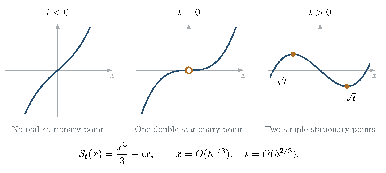
Finally, a degenerate Hessian changes the local model. At a simple fold, two saddles merge. After separating the nondegenerate transverse directions, the remaining phase has the form $$S(x;t)=S_0+\frac{x^3}{3}-tx+\text{higher terms}.$$ The substitution $x=\hbar^{1/3}y$, $t=\hbar^{2/3}s$ gives $$\frac{S-S_0}{\hbar}=\frac{y^3}{3}-sy+\cdots.$$ The resulting contour integral is an Airy integral, rather than a sum of two separately uniform Gaussian approximations. This explains the exponent $2/3$ in the transition scale. For the regular family in Section 15, the real small parameter is $h=2\pi b^2$, so the geometric deformation has scale $b^{4/3}$. When that deformation is proportional to boundary area $A$, the same scale follows from $W\asymp A^{3/2}$ and $W/h=O(1)$. The later theorem proves the contour and additive error estimates for its pole-cleared regular family and fixed bounded real transition parameter. Its volume-action parameter is $\hbar_{\mathrm{vol}}=h/2$ as in (14.24); this constant does not change the exponent $2/3$. The scaling argument alone does not prove a transition theorem. Figure 5 illustrates the cubic normal form and its stationary points; its parameter $t$ is the local fold parameter above.

10.6 Flat connections, Chern–Simons theory, and boundary states

The connection with hyperbolic geometry can be phrased using flat connections. If $\mathscr A$ is a connection one-form, its curvature is $F_{\mathscr A}=\mathop{}\!\mathrm d\mathscr A+\mathscr A\wedge\mathscr A$. In a chosen trivialization the Chern–Simons functional has the form $$\operatorname{CS}(\mathscr A)=\frac1{4\pi}\int_M \mathop{\mathrm{tr}}\left(\mathscr A\wedge\mathop{}\!\mathrm d\mathscr A +\frac23\mathscr A\wedge\mathscr A\wedge\mathscr A\right).$$(10.14) The trace convention fixes the periods and overall normalization. On a closed manifold its first variation is $\delta\operatorname{CS}=(2\pi)^{-1}\int_M \mathop{\mathrm{tr}}(\delta\mathscr A\wedge F_{\mathscr A})$. Thus the critical points are flat connections modulo gauge. The formal expression $\int e^{ik\operatorname{CS}(\mathscr A)}\,D\mathscr A$ motivates the theory; exact algebraic constructions of quantum invariants do not depend on treating this symbol as an ordinary convergent integral [32].

For the compact group $\mathrm{SU}(2)$, the flat connections form the compact character-variety problem. Hyperbolic three-dimensional holonomy instead takes values in $\mathrm{PSL}_2(\mathbb C)$, with a lift to $\mathrm{SL}_2(\mathbb C)$ when chosen. It supplies a distinguished complex flat connection. The correctly normalized complex Chern–Simons action contains both the volume and the Chern–Simons invariant. Analytic continuation and the choice of integration cycle connect these settings; merely changing the name of the gauge group does not specify the cycle [34; 33].

For a manifold with boundary, variation of the functional has a boundary term. This is the source of the symplectic form on boundary flat connections and the need to specify boundary data. Abstractly, a topological quantum field theory assigns a vector space $\mathcal H(\Sigma)$ to an oriented surface, and a vector $\Psi_M\in\mathcal H(\partial M)$ to a three-manifold with boundary. Gluing is a pairing: $$Z(M_1\cup_\Sigma M_2)=\langle\Psi_{M_1},\Psi_{M_2}\rangle,$$ with orientation reversal supplying the dual space and the theory’s framing conventions understood. In finite root-of-unity theories this is finite-dimensional linear algebra. In the analytic models used for complex holonomy, a state is represented locally by a function or distribution of continuous boundary variables, and the pairing becomes an integral. Those analytic models require their own existence and convergence statements.

A polarization chooses which half of the conjugate boundary coordinates are arguments of the state. For a torus boundary, use the multiplier logarithms $u,v$ of Section 16. The Neumann–Zagier normalization is $$\Omega_\partial=\frac12\mathop{}\!\mathrm dv\wedge\mathop{}\!\mathrm du, \qquad \alpha_\partial=\frac12v\,\mathop{}\!\mathrm du.$$(10.15) The geometric deformations of the interior give a Lagrangian curve $v=v(u)$. A semiclassical boundary state associated with this branch has the form $$\Psi_M(u;\hbar)\sim e^{\Phi(u)/\hbar} (a_0(u)+\hbar a_1(u)+\cdots),\qquad \Phi'(u)=\frac12v(u).$$(10.16) The leading exponent is a primitive of the symplectic potential on the Lagrangian curve. This is the geometric content of the WKB (Wentzel–Kramers–Brillouin) ansatz [35].

This choice of half-boundary variables also explains the boundary correction to volume. With $F'=v$ and $F(0)=0$, the note uses $\Phi=\Phi_0+F/2$, with $\Im\Phi_0=V_0$ the complete volume, while $$V(u)-V_0=\frac12\Im F(u)-\frac12\Re u\,\Im v(u).$$(10.17) The last term is essential. The imaginary part of an action in an arbitrary boundary polarization need not itself be the incomplete hyperbolic volume. Section 16.10 derives this identity and the corresponding filling transformation explicitly.

10.7 Quantizing peripheral holonomy and performing surgery

Set $P=v/2$, so that $\Omega_\partial=\mathop{}\!\mathrm dP\wedge\mathop{}\!\mathrm du$. In the formal convention compatible with $e^{\Phi/\hbar}$, use operators $$\widehat u\,\Psi=u\Psi,\qquad \widehat P\,\Psi=\hbar\partial_u\Psi, \qquad [\widehat P,\widehat u]=\hbar.$$(10.18) The usual physical factor $i$ has been absorbed into the parameter $\hbar$; the formula defines the convention here. Acting on the leading exponential gives $\widehat P\Psi\sim\Phi'\Psi=P\Psi$. Thus differentiation becomes the classical longitude coordinate in the small-$\hbar$ limit.

In local eigenvalue coordinates $m=e^{u/2}$ and $l=e^{v/2}$, the corresponding operators are multiplication and translation: $$\widehat m\Psi(u)=e^{u/2}\Psi(u),\qquad \widehat l\Psi(u)=\Psi(u+\hbar),\qquad \widehat l\widehat m=e^{\hbar/2}\widehat m\widehat l.$$ Fixed signs from an $\mathrm{SL}_2$ lift can multiply $m$ and $l$; they do not change this commutation relation. The factor $e^{\hbar/2}$ is the Weyl parameter in these coordinates. It should not be identified with every author’s variable called $q$.

The classical boundary holonomies satisfy a polynomial relation $A(l,m)=0$ on the appropriate character-variety component. To quantize such a relation is to seek a difference operator $\widehat A(\widehat l,\widehat m;\hbar)$ annihilating the boundary state. Substituting (10.16) gives, to leading order, $$A\bigl(e^{\Phi'(u)},e^{u/2}\bigr)=0.$$ This recovers the classical curve because $\Phi'=v/2$. It does not uniquely determine the exact operator: ordering and lower-order terms remain. Identifying a particular operator with a recursion for a particular quantum invariant is a further mathematical statement [34; 35].

Dehn filling has a similarly concrete meaning. For a slope $(p,q)$, choose $\rho,\sigma\in\mathbb Z$ with $p\sigma-q\rho=1$ and put $$a=pu+qv,\qquad b_{\mathrm{core}}=\rho u+\sigma v.$$ Then $\mathop{}\!\mathrm db_{\mathrm{core}}\wedge\mathop{}\!\mathrm da=\mathop{}\!\mathrm dv\wedge\mathop{}\!\mathrm du$. For $q\ne0$ the generating function $$G(u,a)=\frac{pu^2}{4q}-\frac{ua}{2q} +\frac{\sigma a^2}{4q}$$(10.19) satisfies $\mathop{}\!\mathrm dG=\frac12b_{\mathrm{core}}\,\mathop{}\!\mathrm da-\frac12v\,\mathop{}\!\mathrm du$ on this relation. An integral transform with exponential kernel $e^{G/\hbar}$ therefore changes the boundary coordinate from $u$ to $a$. Its stationary equation for $\Phi(u)+G(u,a)$ is exactly $a=pu+qv$. At the classical level, pairing with a solid-torus state imposes the geometric filling branch $a=2\pi i$; the cone-angle family uses $a=i\theta$. The full surgery kernel includes amplitude and topological normalization factors in addition to this exponential.

In the closed-filling convention of this monograph, $\hbar_r=4\pi i/r$. If the filled critical phase has imaginary part $V$, then $$\left|e^{\Phi_{\mathrm{filled}}/\hbar_r}\right| =\exp\left(\frac{rV}{4\pi}\right).$$(10.20) This is the RT exponential in (10.5). After the Fourier-kernel square-root normalization, the Gaussian change of boundary coordinate has dependence $(p+qv'(u))^{-1/2}$, up to its phase; the solid torus contributes further factors. This requires $q\ne0$ in the displayed chart and $p+qv'(u)\ne0$ at the saddle. The calculation in Section 16 makes each of these statements precise and states the hypotheses needed to pass from the geometric contribution to an exact invariant. Notice that the inverse level $r^{-1}$ and the inverse slope length $|p+q\tau|^{-1}$ are independent small parameters; here $\tau=v^\prime(0)$ is the complete cusp shape.

10.8 Liouville theory, conformal blocks, and continuous fusion

Take $0<b<1$. The other quantum construction in this monograph starts in two dimensions. In Liouville theory the variable is a conformal factor $\phi$ on a fixed Riemann surface with reference metric $g$; formally the new area element is $e^{2b\phi}\mathop{}\!\mathrm dA_g$. The field is distributional, so this exponential and its point insertions require renormalization. The Gaussian free field is a generalized Gaussian function with inverse-Laplacian covariance. Gaussian multiplicative chaos constructs its exponential measure by smoothing the field, subtracting half the variance of the scaled field from the exponent, and taking a limit. In the subcritical range above this gives the rigorous random measures used here [68].

The basic observables are the renormalized exponential insertions $V_\alpha(p)\sim e^{2\alpha\phi(p)}$. A correlation function is the averaged product $$C_b(\boldsymbol\alpha;\boldsymbol p) =\left\langle\prod_i V_{\alpha_i}(p_i)\right\rangle.$$ It depends on the marked conformal surface. It is neither a three-manifold invariant nor, without a further operation, a measure on moduli space. The parameters governing conformal symmetry are $$Q=b+b^{-1},\qquad c_L=1+6Q^2,\qquad \Delta(\alpha)=\alpha(Q-\alpha).$$(10.21) Here $c_L$ is the central charge and $\Delta$ the conformal weight. Concretely the infinitesimal symmetry algebra is the Virasoro algebra $$[L_m,L_n]=(m-n)L_{m+n} +\frac{c_L}{12}(m^3-m)\delta_{m+n,0}.$$ A highest-weight vector has $L_0$-eigenvalue $\Delta$ and is killed by $L_n$ for $n>0$; its descendants are obtained with the negative generators. This representation theory determines the power series called conformal blocks [95].

On a four-marked sphere with marks $0,1,z,\infty$, a pants decomposition first combines two of the insertions. Fixing the intermediate representation with label $\alpha_s$ gives a chiral conformal block: a holomorphic, generally multivalued function with a specified leading behavior, for example $$\mathcal F^{(s)}_{\alpha_s}(z) =z^{\Delta(\alpha_s)-\Delta(\alpha_1)-\Delta(\alpha_3)} (1+O(z)).$$ “Chiral” refers here to the holomorphic half. The full correlation pairs holomorphic and antiholomorphic blocks and integrates over the intermediate spectrum. Label the insertions at $0,1,z,\infty$ by $\alpha_1,\alpha_2,\alpha_3,\alpha_4$, respectively. For real external charges in the initial domain $\alpha_i<Q/2$, $\alpha_1+\alpha_3>Q/2$, and $\alpha_2+\alpha_4>Q/2$, the proved four-point decomposition has the form $$C_b(z,\bar z)=\int_0^\infty \rho(\alpha_1,\ldots,\alpha_4;P)\, |\mathcal F^{(s)}_{Q/2+iP}(z)|^2\,\mathop{}\!\mathrm dP,$$ with normalization and products of three-point structure constants included in $\rho$. The explicit three-point constants are the DOZZ constants, named for Dorn–Otto and Zamolodchikov–Zamolodchikov. The relevant three-point formula and four-point decomposition have rigorous constructions and proofs in their stated domains [68; 60]. Here the charges in [60, Theorem 1.1] are twice our $\alpha_i$. Continuing outside that domain can require additional residues when poles cross the spectral contour. For complex charges the two chiral factors must be continued analytically in the charges; the real-domain absolute-square notation does not prescribe that continuation.

Changing the pants decomposition gives the fusion kernel: $$\mathcal F^{(s)}_{\alpha_s}(z) =\int_{\mathcal C} F_{\alpha_s\alpha_t}\, \mathcal F^{(t)}_{\alpha_t}(z)\,\mathop{}\!\mathrm d\alpha_t.$$(10.22) The measure is either displayed separately or incorporated in $F$. This is the continuous counterpart of (10.1): four external labels and two internal ones again give six labels. Rescaling the basis blocks changes the displayed kernel. Accordingly the fusion kernel is related to a $b$-$6j$ symbol through explicit trivalent normalization and spectral factors, not by an unqualified equality of scalar functions [96, Section 4].

The noncompact representation theory behind this kernel is the modular double. It uses the compatible deformation parameters $$q_{\mathrm{alg}}=e^{\pi i b^2},\qquad \widetilde q_{\mathrm{alg}}=e^{\pi i/b^2}.$$ The principal representation labels are $\alpha=Q/2+iP$; tensor products decompose by direct integrals instead of finite sums. The double refers to the simultaneous roles of $b$ and $b^{-1}$. The corresponding $b$-$6j$ is a continuous recoupling kernel. This is a different setting from the finite root-of-unity label set in Section 10.1.

Its explicit formulas use Barnes’ double Gamma function $\Gamma_b$, a meromorphic analogue of the Gamma function with the two step sizes $b$ and $b^{-1}$, and the double sine $$S_b(x)=\frac{\Gamma_b(x)}{\Gamma_b(Q-x)},\qquad \begin{aligned} S_b(x+b)&=2\sin(\pi bx)S_b(x),\\ S_b(x+b^{-1})&=2\sin(\pi x/b)S_b(x),\\ S_b(x)S_b(Q-x)&=1. \end{aligned}$$(10.23) These identities explain why sine factors and pole movements occur in the later calculations. The double sine is related to Faddeev’s noncompact quantum dilogarithm by shifted arguments and explicit Gaussian factors; conventions matter [96, Appendix A].

The first shift relation also explains its classical limit. Put $L_b(x)=b^2\log S_b(x/b)$ for real $x$ in the fundamental strip. Then $$L_b(x+b^2)-L_b(x)=b^2\log(2\sin\pi x).$$ A smooth leading limit must therefore have derivative $\log(2\sin\pi x)$. Reflection fixes the constant, giving $L(x)=-\Lambda(\pi x)/\pi$ for $0<x<1$. This is a formal derivation of the leading term; Lemma 15.2 supplies the uniform estimate used in the proof. Thus the same Lobachevsky function that appeared in the elementary figure-eight sum also appears in the continuous $b$-$6j$ analysis.

10.9 Why a screening residue meets flat cone geometry

The particular Liouville specialization in this monograph can be understood through a one-variable integral. Separate the constant part $c_0$ of the field from its nonconstant part. After the insertions have shifted the Gaussian field, let $Z>0$ be the remaining random area factor and put $$s=\frac{\sum_i\alpha_i-Q}{b}.$$ With the overall normalization adopted in (12.2), the integral over the constant mode is $$2\int_{\mathbb R}e^{2bs c_0-\Lambda_L Z e^{2bc_0}}\,\mathop{}\!\mathrm dc_0 =\frac1b\Lambda_L^{-s}\Gamma(s)Z^{-s},\qquad \Re s>0.$$(10.24) This is just the substitution $t=\Lambda_L Z e^{2bc_0}$. The positive number $\Lambda_L$ is the cosmological constant, or coefficient penalizing total area. The formula explains both the Gamma factor in the correlation and the usefulness of removing that factor in the unit-volume normalization.

Now take the deficit weights of the flat cone metric: $$0<\mu_i<1,\quad \sum_i\mu_i=2,\qquad \alpha_i=\frac{\mu_i}{2b}.$$ Then $\sum_i\alpha_i=1/b=Q-b$, and therefore $s=-1$. The raw integral (10.24) does not converge there. Its meromorphic continuation has a Gamma pole, whereas the continued unit-volume expression contains $Z^{-s}=Z$: its first moment. The normalized random measure has the prescribed reference measure as its expectation. The reference factors cancel at these weights, leaving, in a coordinate with all marks finite, $$\mathbb E[Z]=\mathcal A_\mu(\boldsymbol p) =\int_{\mathbb C}\prod_i|w-p_i|^{-2\mu_i}\,\mathop{}\!\mathrm d^2w.$$(10.25) This is precisely the area of the flat cone metric that underlies the Thurston–Deligne–Mostow construction. The charge convention in the detailed probabilistic formulas is $\beta_i=2\alpha_i$. Section 12 checks the continuation and integrability conditions and proves the exact finite-$b$ identity.

The remaining factors in the correlation are pairwise powers of $|p_i-p_j|$, whose logarithms are pluriharmonic away from collisions. Consequently the operation that produces the geometric form is $$-2i\,\partial\bar\partial\log C_b^{\mathrm{uv}} =\omega_{\mathrm{CH},\mu},\qquad \mathop{}\!\mathrm dV_{\mathrm{CH},\mu} =\frac{\omega_{\mathrm{CH},\mu}^{n-3}}{(n-3)!}.$$(10.26) The correlation supplies a logarithmic potential; its logarithmic curvature supplies the form; the top exterior power supplies the moduli measure. These are three different operations. This is why the exact comparison does not identify an unmodified quantum amplitude with a WP or complex hyperbolic volume density.

The name one screening has an equally concrete explanation. The insertion $V_b$ has conformal weight $\Delta(b)=b(Q-b)=1$, so integrating it gives a conformally covariant insertion. At $\sum_i\alpha_i=Q-b$, one such insertion balances the background charge. Its chiral contour integrals are $$\int_\gamma\prod_i(w-p_i)^{-\mu_i}\,\mathop{}\!\mathrm dw,$$ the Deligne–Mostow periods. For four points the relevant twisted period space is two-dimensional, and changing contour bases gives the finite hypergeometric fusion matrix calculated in Section 13. Generic Liouville fusion is still the integral operator (10.22); the $2\times2$ matrix is the exact change of basis for these finite periods. Identifying it with a residue of the continued infinite fusion operator also requires the spectral-continuation and tail input stated in Section 13. The first-moment area identity does not require that additional spectral input. At balanced weights a logarithmic basis is needed. The auxiliary tetrahedron also need not be the convex realization of the original cone sphere. Section 14 checks that geometric comparison separately.

10.10 Parameters, limits, and a route through the calculations

The notation records several independent limits. The following dictionary prevents a formal resemblance of symbols from identifying different asymptotic questions.

The last charge prescription is the pure heavy-charge scaling: the labels grow like $b^{-1}$ while the deficit weights stay fixed. The exact length-kernel dictionary has additional finite-$b$ shifts, recorded in (12.22). Fixed labels with $q\to1$, labels growing with the order of a root of unity, and the continuous $b\to0$ limit are different problems. The classical large-spin $6j$ asymptotic involves Euclidean tetrahedra [91]; particular compact root regimes involve spherical tetrahedra [26]; the hyperbolic regimes used below have their own label and contour hypotheses. Geometric edge lengths or angles are assigned only after specifying the relevant regime.

The quantum part of this monograph can now be read along three routes. For the boundary-moduli comparison, begin with Section 12, then follow the four-point residue and its normalization in Sections 13 and 14. For the degeneration of an individual tetrahedron, use Section 11, the regular family in Section 14, and the uniform theorem for the cleared regular-family integral at bounded real Airy parameter in Section 15. For three-manifold volume and surgery, Section 16 is largely independent of the Liouville calculations; its symplectic explanation is in Section 16.10.

An exact identity of kernels, a local saddle expansion, and a theorem about a global invariant answer different questions. The later sections state which one is obtained at each step. This distinction permits the geometric calculations to be used fully without silently assuming an integration cycle, a measure on moduli, or a dominance theorem that has not been established.