28 Genus two: compact polyhedra and a marked-torus model

28.1 Six branch points and the compact polyhedron

Every genus-two Riemann surface $X$ is hyperelliptic. Its quotient map $\pi:X\to\mathbb P^1$ has six branch values: the Riemann–Hurwitz formula reads $2=2(-2)+6$. With compatible markings the quotient induces a holomorphic Teichmüller isometry $$\mathcal T_{2,0}\cong\mathcal T_{0,6};$$ see, for example, [101, Corollary 1.2(3)]. Both sides have complex dimension three. The four-pointed sphere is the corresponding genus-one example.

The hyperelliptic involution is an isometry of the curvature-$-1$ metric on $X$. The quotient metric is a hyperbolic sphere with six cone angles $\pi$, and its area is $2\pi$. Alexandrov’s hyperbolic realization theorem therefore gives a unique compact convex polyhedron in $\mathbb H^3$ whose intrinsic boundary metric is this quotient metric, allowing the usual degenerate case of a doubled convex polygon [102, Theorem 1.1]. There are six vertices, all with intrinsic total angle $\pi$. Conversely, take the double cover of such a cone sphere branched at its six vertices. Each cone angle becomes $2\pi$, so the lifted metric is smooth, complete, and of curvature $-1$. Riemann–Hurwitz identifies its genus as two. Thus this compact-polyhedral realization is an exact model for the genus-two hyperbolic metric, with the appropriate finite labeling and marking conventions.

This metric must be distinguished from the complete hyperbolic metric on the sphere with the six branch values deleted. The latter has six cusps and area $8\pi$; it is the metric to which the ideal-polyhedron realization applies. Passing between them uses uniformization within the same punctured conformal class. It does not identify their lengths, vertex data, or volume forms. In particular, fixed intrinsic cone angles at compact vertices are not automatically linear constraints on the dihedral angles.

28.2 An explicit formula for every quadratic differential

Choose a coordinate with all six branch values finite and write $$X:\quad y^2=B_6(z):=\prod_{i=1}^{6}(z-a_i).$$(28.1) The forms $\mathop{}\!\mathrm dz/y$ and $z\mathop{}\!\mathrm dz/y$ form a basis of $H^0(X,K_X)$. Their three symmetric products are linearly independent and, by Riemann–Roch, span $H^0(X,K_X^2)$. Hence every holomorphic quadratic differential is $$q_X=P_2(z)\frac{\mathop{}\!\mathrm dz^2}{y^2} =\pi^*q_0, \qquad q_0=\frac{P_2(z)}{B_6(z)}\mathop{}\!\mathrm dz^2, \qquad \deg P_2\leq2.$$(28.2) In particular, every such differential is invariant under the hyperelliptic involution. At a branch point the order transforms by $$\operatorname{ord}_p(\pi^*q_0) =2\operatorname{ord}_{\pi(p)}(q_0)+2.$$(28.3) For a generic polynomial with two distinct roots away from the branch values, this gives $$\mathcal Q_2(1^4)\longleftrightarrow \mathcal Q_0(1^2,-1^6),$$ with finite choices of labels understood. This is the genus-two case of the hyperelliptic covering construction in [103, Section 1.1.3]. The descended flat metric has six angles $\pi$ at its poles and two angles $3\pi$ at its zeros. It is different from the hyperbolic cone metric of the preceding subsection.

Pullback multiplies flat area by two. Thus the correspondence between unit-area differentials on the six-pointed sphere and on $X$ is $$q_0\longmapsto\tfrac12\pi^*q_0.$$ It commutes with $g_t=\mathop{\mathrm{diag}}(e^t,e^{-t})$, with no change of the time parameter. Period-lattice covolumes, finite labelings, and orbifold stabilizers must still be tracked when comparing unnormalized Masur–Veech volumes; the area factor alone is not a formula for those volumes.

28.3 The nonsquare stratum with two double zeros

Write $\mathcal Q^{\mathrm{ns}}_2(2,2)$ for quadratic differentials with two double zeros which are not global squares of Abelian differentials. The superscript is essential: the squares of differentials in $\mathcal H_2(1,1)$ have the same quadratic zero orders but form a different locus.

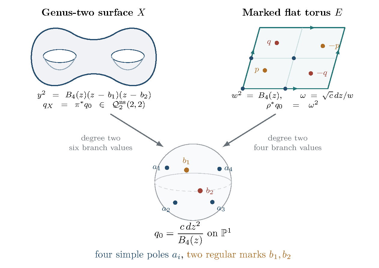
Formula (28.2) gives an elementary description. The differential is a global square exactly when $P_2$ is the square of a polynomial of degree at most one: this follows by writing every Abelian differential as $(az+b)\,\mathop{}\!\mathrm dz/y$. In homogeneous degree-two notation this includes a double root at infinity. A nonzero constant $P_2$ is therefore a square, while a degree-one $P_2$ has a simple zero at each of the two unbranched points at infinity and cannot lie in $\mathcal Q_2(2,2)$. For degree two, a simple root at a branch value gives one double zero by (28.3), and a simple root elsewhere gives two simple zeros. Thus, to obtain two double zeros without a square, the roots must be two distinct branch values, say $b_1,b_2$. After relabeling the remaining four branch values, $$\begin{split} X:&\quad y^2=B_4(z)(z-b_1)(z-b_2), \qquad B_4(z)=\prod_{i=1}^4(z-a_i),\\ q_X&=c(z-b_1)(z-b_2)\frac{\mathop{}\!\mathrm dz^2}{y^2} =\pi^*\left(\frac{c\,\mathop{}\!\mathrm dz^2}{B_4(z)}\right), \qquad c\in\mathbb C^*. \end{split}$$(28.4) The six values $a_1,\ldots,a_4,b_1,b_2$ are distinct. Downstairs $q_0=c\,\mathop{}\!\mathrm dz^2/B_4(z)$ has four simple poles and is regular at the two additionally marked points $b_1,b_2$: $$\mathcal Q^{\mathrm{ns}}_2(2,2) \longleftrightarrow \mathcal Q_0(-1^4,0,0).$$(28.5) The regular marks cannot be discarded. They are branch values of $X\to\mathbb P^1$, and their positions supply four real parameters.

For each fixed $X$, choosing the unordered pair of branch values $b_1,b_2$ gives $\binom62=15$ complex lines of nonsquare $(2,2)$ differentials in the three-dimensional cotangent space. Area normalization leaves a phase on each line. Consequently this stratum meets every conformal base, but its unit-area locus has real dimension seven, compared with eleven for the full principal unit cotangent locus. Its Masur–Veech measure is an intrinsic stratum measure, not a conditional probability obtained by restricting the principal measure to a set of measure zero.

28.4 The pillowcase cover and two marked torus points

The orientation double cover of the four-pole differential $q_0$ is the elliptic curve $$E:\quad w^2=B_4(z), \qquad \omega=\sqrt c\,\frac{\mathop{}\!\mathrm dz}{w}, \qquad \rho^*q_0=\omega^2.$$(28.6) Choose one branch point of $E\to\mathbb P^1$ as the origin. The involution is then $v\mapsto-v$, and its four fixed points are $E[2]$. The two marked regular points lift to unordered pairs $$\rho^{-1}(b_1)=\{p,-p\},\qquad \rho^{-1}(b_2)=\{q,-q\}.$$ Their admissibility conditions are exactly $$p,q\notin E[2],\qquad p\ne q,\qquad p\ne -q.$$(28.7) Conversely, a flat torus $(E,\omega)$ with an origin and such two points gives the sphere $E/\{\pm1\}$ with its four poles and two regular marks. The unique connected double cover of this sphere branched at all six marked values is $X$, and pullback of $q_0$ gives (28.4). The cover is connected because its monodromy is the nontrivial homomorphism to $\mathbb Z/2\mathbb Z$ on every small loop around a branch value; six such loops satisfy the sphere relation. It is unique because those loops generate the fundamental group of the punctured sphere.

The resulting $q_X$ is nonsquare. Indeed, its being square would force the orientation cover $E\to\mathbb P^1$ to factor through $X\to\mathbb P^1$. Both covers have degree two, but their branch sets differ: the former is branched at the four $a_i$, the latter also at $b_1,b_2$. Equivalently, the square root of $B_4$ is not in the function field $\mathbb C(z,\sqrt{B_4(z)(z-b_1)(z-b_2)})$.

Both covering maps to the sphere have degree two, so $$\operatorname{Area}(E,\omega) =2\operatorname{Area}(q_0) =\operatorname{Area}(X,q_X).$$(28.8) Thus the unit-area marked torus corresponds directly to the unit-area genus-two differential, with no further area scaling. The entire construction commutes with the $SL_2(\mathbb R)$ action on flat charts. In particular its time parameter is exactly the Teichmüller time used above. Figure 8 records the distinct branch sets of the two covers and the two lifted pairs of regular marks.

28.5 A homogeneous finite cover

Choose a full symplectic level-two structure on the torus and choose an ordering and one lift from each of the two pairs $\{\pm p\},\{\pm q\}$. Together with the origin, level two labels the four two-torsion points and hence the four poles. Set $$\Gamma_2=\ker\bigl(SL_2(\mathbb Z)\to SL_2(\mathbb Z/2\mathbb Z)\bigr), \qquad G_2=SL_2(\mathbb R)\ltimes(\mathbb R^2\oplus\mathbb R^2),$$ where $SL_2(\mathbb R)$ acts in the standard way on both vector factors. Our group law and right-quotient convention are $$\begin{aligned} (A,u_1,u_2)(B,v_1,v_2) &=(AB,u_1+Av_1,u_2+Av_2),\\ Y_2&=G_2/(\Gamma_2\ltimes(\mathbb Z^2\oplus\mathbb Z^2)). \end{aligned}$$ A representative $(A,u_1,u_2)$ describes the area-one torus $\mathbb R^2/A\mathbb Z^2$ with marked points $[u_1],[u_2]$. Right multiplication by $(\gamma,n_1,n_2)$ changes the representative to $$(A\gamma,u_1+An_1,u_2+An_2),$$ which is exactly change of the lattice basis preserving level two and change of the two point lifts. The presence of $-I$ in $\Gamma_2$ causes no singularity in this homogeneous quotient: right translation by a discrete subgroup on a Lie group is free. Here $A$ and $-A$ give the same physical lattice and the same level-two data. A finer congruence level gives an additional finite cover. The spectral argument below uses level two specifically; its conclusion about the base spectrum is not automatically inherited by further covers.

Delete the locus where one of the points is two-torsion or where $[u_1]=\pm[u_2]$, and call the resulting open set $Y_2^\circ$. In each torus fiber the deleted set is a finite union of real codimension-two subtori. It has Haar measure zero and its complement is connected. Since the base $SL_2(\mathbb R)/\Gamma_2$ is connected, so is $Y_2^\circ$. Forgetting the finite marking choices gives a finite equivariant local parameterization of $\mathcal Q^{\mathrm{ns},1}_2(2,2)$. The finite choices include the distinguished origin over a pole, the level structure, the ordering of the two regular marks, and their signs. Their changes preserve Haar measure and commute with the $SL_2(\mathbb R)$ action; the stratum is their finite quotient. Over the coarse-moduli locus without additional automorphisms this is an ordinary finite covering. If one retains the ubiquitous genus-two hyperelliptic involution in the orbifold stabilizers, its fixed order-two contribution must also be included in unnormalized volume conventions. No infinite marking choice is being discarded in this finite-cover statement.

The flow is left multiplication: $$g_t[A,u_1,u_2] =[a_tA,a_tu_1,a_tu_2], \qquad a_t=\mathop{\mathrm{diag}}(e^t,e^{-t}).$$(28.11) The admissible set $Y_2^\circ$ is invariant under this action. Although the coordinates $\xi_i=A^{-1}u_i\pmod{\mathbb Z^2}$ are unchanged in a fixed lattice chart, a change $A\mapsto A\gamma$ changes them by $\xi_i\mapsto\gamma^{-1}\xi_i$. Therefore they are not globally fixed torus coordinates on the quotient. This monodromy is essential in the later Fourier calculation.

28.6 Haar measure and the period lattice

The group $G_2$ is unimodular, and its Haar measure is $$\mathop{}\!\mathrm dA\,\mathop{}\!\mathrm du_1\,\mathop{}\!\mathrm du_2,$$ where $\mathop{}\!\mathrm dA$ is Haar measure on $SL_2(\mathbb R)$. In a local lattice chart, $u_i=A\xi_i$ and $\det A=1$, so its quotient measure is the product of modular Haar measure and Lebesgue probability on $(\mathbb R^2/\mathbb Z^2)^2$. The modular quotient has finite Haar volume and each torus fiber has volume one, hence $Y_2$ has finite volume.

Before area normalization, local coordinates are the two complex lattice periods and the two complex positions of the marked points. These are four complex coordinates, agreeing with $$\dim_{\mathbb C}\mathcal Q^{\mathrm{ns}}_2(2,2)=4.$$ The covering construction transports these coordinates to quadratic-differential period coordinates by a fixed linear map on each marked chart. This can be seen without a global classification theorem. The orientation cover of $q_X$ is the fiber product $$\widehat X:\quad w^2=B_4(z),\qquad t^2=(z-b_1)(z-b_2), \qquad y=wt, \qquad \widehat\omega=\sqrt c\,\frac{\mathop{}\!\mathrm dz}{w}.$$ Its map to $E$ is a double cover branched at $\{p,-p,q,-q\}$. Thus its relative periods are integral linear combinations of torus periods and marked-point positions, after paths and lifts have been fixed. Transfer on absolute cycles and paths between $p$ and $-p$, or between $q$ and $-q$, recover the torus periods and twice the point positions, up to periods. Consequently the inverse change of coordinates is rational linear. The integral period lattices are commensurable; factors of two can occur, so the map need not be unimodular. This is the period-coordinate construction underlying the stratum measure [103, Sections 1.1.1–1.1.2].

It follows that the transported Masur–Veech measure is a constant multiple of Lebesgue measure in these cone coordinates. More explicitly, write the torus area as $s>0$, put $A=\sqrt{s}\,B$ with $\det B=1$, and use the point coordinates $\xi_i=A^{-1}u_i$. Up to a fixed positive constant the cone measure is $$s^3\,\mathop{}\!\mathrm ds\,\mathop{}\!\mathrm dB\,\mathop{}\!\mathrm d\xi_1\,\mathop{}\!\mathrm d\xi_2.$$ Restricting by area as in (28.8) therefore makes the unit-area measure a constant multiple of Haar measure on $Y_2$. After normalizing to probability and accounting for the finite covering, the measures agree. No numerical identity between unnormalized volumes is asserted without a choice of lattice and labeling conventions. The measure-zero exclusions in $Y_2\setminus Y_2^\circ$ do not affect this probability identification.

For observables compactly supported inside $Y_2^\circ$, extension by zero gives smooth observables on the homogeneous space. Thus estimates proved there pass to the stratum after lifting the observables and, if necessary, averaging over the finite markings. For observables which grow near collisions, extension and norm control require additional estimates; a null collision set alone is not a bound on such observables.

28.7 Fourier decomposition and temperedness

The affine homogeneous model admits a direct calculation which does not use a general Teichmüller mixing theorem. Let $$G=\operatorname{SL}_2(\mathbb R),\qquad \mathsf A=G\ltimes\operatorname{Mat}_{2\times2}(\mathbb R),\qquad \Lambda=\Gamma\ltimes\operatorname{Mat}_{2\times2}(\mathbb Z),$$ where $\Gamma=\Gamma(2)$ initially. The group law is $$(g,v)(g',v')=(gg',v+gv').$$ Set $Y_2=\mathsf A/\Lambda$, with Haar probability measure $\mu$, and let $a_t=\mathop{\mathrm{diag}}(e^t,e^{-t})$ act by left translation. A point is a unit-area lattice together with two marked vectors modulo that lattice. If one counts the origin as a marked point, this is a torus with three ordered marked points. Coincidence loci have measure zero and may be removed. Any application to a particular quadratic stratum uses its separately established geometric identification with this model or a finite quotient; an arbitrary finite cover cannot be discarded without checking its base spectrum.

28.8 A global correlation bound with an explicit constant

Let $K=\operatorname{SO}(2)$, with angular generator $\Theta$, normalized so that the $n$th character has derivative $in$. Use the norm $$\mathcal S_1(F)^2=\|F\|_2^2+\|\Theta F\|_2^2.$$(28.16) The angle is the ordinary matrix rotation angle: on the orientation cover, $\omega$ changes to $e^{i\theta}\omega$, so the genus-two quadratic differential changes to $e^{2i\theta}q_X$. Thus this normalization is twice differentiation in the phase of $q_X$. Write $F^\circ=F-\mu(F)$ and $G^\circ=G-\mu(G)$. The Cowling–Haagerup–Howe bound for a tempered representation is $$|\langle\pi(g)v,w\rangle| \leq\Xi(g)\|v\|\|w\| \sqrt{\dim Kv\,\dim Kw}$$ for $K$-finite vectors; see [105, Proposition 2.6] and [106]. For single $K$-types the two dimension factors equal one. Decomposing into $K$-types and using Cauchy–Schwarz gives $$\sum_{n\in\mathbb Z}\|F_n\|_2 \leq\left(\sum_{n\in\mathbb Z}(1+n^2)^{-1}\right)^{1/2} \mathcal S_1(F) =\sqrt{\pi\coth\pi}\,\mathcal S_1(F).$$ Here the subscript denotes $K$-type, distinct from the matrix frequency in (28.12).

For $e_1=(1,0)^T$, the spherical principal-series realization gives $\Xi(a_t)=\int_K|a_tke_1|^{-1}\,\mathop{}\!\mathrm dk$, with Haar probability on $K$. Using $u=\tan\theta$ on a quadrant gives, in our time normalization, the elementary integral $$\Xi(a_t)=\frac2\pi e^{-t} \int_0^\infty \frac{\mathop{}\!\mathrm du}{\sqrt{(1+u^2)(1+e^{-4t}u^2)}} \leq\frac4\pi(1+t)e^{-t},\qquad t\geq0.$$(28.17) For the inequality, split the integral at $u=1$ and $u=e^{2t}$. The three contributions are at most $1$, $2t$, and $1$.

Centering the functions does not increase $\mathcal S_1$. The norm needs only one rotation derivative; neither derivatives in the marked-point coordinates nor compact support are required. This is global on the finite-volume affine quotient. No compact cutoff or unquantified cusp-tail estimate enters this inequality. The polynomial factor allows every pure exponential rate $e^{-(1-\varepsilon)t}$, but not a uniform constant times $e^{-t}$ from this argument. More explicitly, for $0<\varepsilon\leq1$ one may replace $4\coth\pi(1+t)e^{-t}$ by $4\coth\pi\,\varepsilon^{-1}e^{-(1-\varepsilon)t}$. For the convention $a_t=\mathop{\mathrm{diag}}(e^{t/2},e^{-t/2})$, replace $t$ by $t/2$ throughout.

28.9 An exact finite lattice sum with two endpoint weights

The following unfolding supplies a concrete counting statistic. For $\varphi,\psi\in C_c^\infty(\mathsf A)$ let $$P\varphi(h\Lambda)=\sum_{\lambda\in\Lambda}\varphi(h\lambda), \qquad F=P\varphi,\quad G=P\psi.$$ Normalize Haar measure $\mathop{}\!\mathrm dh$ so that $\mathsf A/\Lambda$ has volume one. For fixed $t$ define the overlap weight $$W_t^{\varphi,\psi}(\lambda) =\int_{\mathsf A}\overline{\varphi(h)}\, \psi(a_th\lambda)\,\mathop{}\!\mathrm dh.$$(28.19) Only finitely many $\lambda$ contribute, since any such lattice element lies in the compact set $(\operatorname{supp}\varphi)^{-1}a_{-t} \operatorname{supp}\psi$. In coordinates $h=(g,v)$ and $\lambda=(\gamma,m)$, the weight is explicitly $$W_t^{\varphi,\psi}(\gamma,m) =\int_G\int_{\operatorname{Mat}_{2\times2}(\mathbb R)} \overline{\varphi(g,v)}\, \psi\bigl(a_tg\gamma,a_t(v+gm)\bigr)\,\mathop{}\!\mathrm dv\,\mathop{}\!\mathrm dg.$$(28.20) Unfolding the periodization of the first observable gives exactly $$\sum_{\lambda\in\Lambda}W_t^{\varphi,\psi}(\lambda) =\int_{Y_2}\overline F\,(G\circ a_t)\,\mathop{}\!\mathrm d\mu.$$(28.21) The weights are nonnegative when $\varphi$ and $\psi$ are nonnegative. For arbitrary observables they are signed or complex. Thus (28.21) is a finite weighted return sum, not an assertion about an unweighted sharp orbit count.

The unstable Jacobian exponent is $4$: conjugation by $a_t$ expands the upper-unipotent direction in $\mathfrak{sl}_2$ by $e^{2t}$ and the two expanding translation directions by $e^t$ each. Accordingly define the normalized return statistic and its cumulative version, for $T\geq1$, by $$\mathcal N_{\varphi,\psi}(t) =e^{4t}\sum_{\lambda\in\Lambda} W_t^{\varphi,\psi}(\lambda),\qquad \mathcal A_{\varphi,\psi}(T) =\int_1^T\mathcal N_{\varphi,\psi}(t)\,\mathop{}\!\mathrm dt.$$ This normalization uses the affine model’s unstable Jacobian. It does not use the polar Jacobian of full Teichmüller space. Since $\mu(P\varphi)=\int_{\mathsf A}\varphi\,\mathop{}\!\mathrm dh$, (28.18) gives the explicit remainder $$\begin{split} \left|\mathcal A_{\varphi,\psi}(T) -\overline{\mu(F)}\mu(G)\frac{e^{4T}-e^4}{4}\right| \leq\frac43\coth\pi\,(1+T)e^{3T} \mathcal S_1(F^\circ)\mathcal S_1(G^\circ). \end{split}$$(28.22) Equivalently, with $R=e^T$, this is an $O(R^3\log R)$ remainder against an $R^4$ main term, with a displayed norm bound. Here $R=e^T$ is an exponential-time parameter; identifying it with hyperbolic curve length, intersection number, or square-tiled area would require a separate comparison. The estimate follows simply from $\int_1^T(1+t)e^{3t}\mathop{}\!\mathrm dt\leq\tfrac13(1+T)e^{3T}$.

These norms can also be bounded using the original compactly supported weights. If $K_0\subset \mathsf A$ contains their supports and $$M_{K_0}=\#(\Lambda\cap K_0^{-1}K_0),$$ then Cauchy–Schwarz in the locally finite periodization gives $$\mathcal S_1(P\varphi) \leq\sqrt{M_{K_0}} \bigl(\|\varphi\|_{L^2(\mathsf A)}^2+ \|\Theta\varphi\|_{L^2(\mathsf A)}^2\bigr)^{1/2},$$ and similarly for $\psi$. All quantities in this bound are finite for the chosen compact supports.

Define the flow generator by $V\psi(h)=\left.\frac{\mathop{}\!\mathrm d}{\mathop{}\!\mathrm ds}\right|_{s=0}\psi(a_sh)$. Periodization commutes with this generator: $V(P\psi)=P(V\psi)$. Therefore inserting the terminal weight $(4+V)\psi$ gives the exact identity $$\begin{split} \mathcal A_{\varphi,(4+V)\psi}(T) &=e^{4T}\int_{Y_2}\overline F\,(G\circ a_T)\,\mathop{}\!\mathrm d\mu\\ &\quad-e^4\int_{Y_2}\overline F\,(G\circ a_1)\,\mathop{}\!\mathrm d\mu. \end{split}$$(28.23) There is no convolution operator to commute past $V$, and no unjustified differentiation of a counting asymptotic. The quantitative norm required for this terminal test is $\mathcal S_1((4+V)G)\leq4\mathcal S_1(G)+\mathcal S_1(VG)$. It includes $\|\Theta VG\|_2$; the generators $\Theta$ and $V$ do not commute, and this mixed derivative is not omitted.

28.10 What the marked-torus calculation settles

The compact polyhedron encodes the genus-two hyperbolic base, whereas the marked flat torus encodes the nonsquare $(2,2)$ differential and its flow. They use different intrinsic metrics and are linked by the same six branch values. The affine model gives an exact Fourier decomposition, an explicit global correlation bound, and the finite weighted return sum with remainder (28.22). These are conclusions of the calculation, not hypotheses imported from general Teichmüller mixing. The inputs are classical: amenability and induction, the Cowling–Haagerup–Howe bound, the elementary $SL_2$ spherical function, and the absence of positive small spectrum on the thrice-punctured sphere. Related marked-torus harmonic analysis is already developed in [104; 108]; no novelty claim for that machinery is intended.

The derivative identity (28.23) also makes the counting converse exact in this model. After subtracting the product of means, a bound for the terminal test $(4+V)G$ recovers the correlation at $T$ with the same exponential saving. In the proof here the direction is Fourier/representation theory to correlations and hence to counts. The identity identifies the reverse implication as well, without making the proof circular.

The restriction to the chosen stratum remains substantial. Although it meets every genus-two conformal base, its unit-area dimension is seven; the principal unit stratum has dimension eleven. The affine expanding Jacobian is $e^{4t}$, whereas the full genus-two Teichmüller polar kernel in Section 27 has exponent $6$. The two kernels cannot be substituted for one another. Section 29 constructs selected primitive-arc observables from the coefficient data with controlled geometric norms. A comparison with the full orbit kernel, and uniform stability of the nonlinear coefficient extraction, remain open. In particular, the $O(R^3\log R)$ estimate above is not an error term for the unweighted count of connected simple closed geodesics. A comparison with that count, or an extension to the principal stratum $\mathcal Q^1_2(1^4)$, is a further problem.