30 Diagnosing the sharp remainder without fitting its main term

30.1 The normalized all-point discrepancy and the logarithmic loss

Let $B$ be a fixed convex body containing the origin in its interior. Rescale its gauge so that the shortest nonzero integer vector has gauge one; central symmetry is not needed in this subsection. Write $a=\operatorname{Area}(B)$, $$A_0(u)=\#(uB\cap(\mathbb Z^2\setminus\{0\})),\qquad D_B(u)=A_0(u)-a u^2,$$ and let $P_B(L)$ count primitive vectors. For $M=\lfloor L\rfloor$, Möbius inversion gives the exact identity $$\frac{P_B(L)-aL^2/\zeta(2)}{L} =\sum_{d\le M}\frac{\mu(d)}d\, \frac{D_B(L/d)}{L/d} -aL\sum_{d>M}\frac{\mu(d)}{d^2}.$$(30.1) The cutoff is exact because $A_0(u)=0$ for $u<1$; boundary points at $u=1$ are included. Moreover $L\sum_{d>M}d^{-2}\le L/M\le2$ for $L\ge2$, so the final term is bounded uniformly. Thus the linear remainder problem is precisely a boundedness problem for the displayed Möbius-weighted harmonic sum. The prime number theorem alone does not bound it: the geometric weight $D_B(L/d)/(L/d)$ varies with both $L$ and $d$.

For a convenient sufficient condition, put $$\omega_B(u)=\sup_{v\ge u}\frac{|D_B(v)|}{v},\qquad u\ge1.$$ The elementary boundary estimate makes $\omega_B$ bounded, and it is nonincreasing. Absolute values in (30.1) give $$|P_B(L)-aL^2/\zeta(2)| \le C_B L\left(1+\int_1^L\omega_B(u)\,\frac{du}{u}\right).$$(30.2) Indeed, for $d\le M$, $$\int_{L/(d+1)}^{L/d}\omega_B(u)\frac{du}{u} \ge\omega_B(L/d)\log(1+1/d) \ge\frac{\omega_B(L/d)}{2d},$$ with the harmless interval below $1$ treated separately. Consequently the Dini condition $$\int_1^\infty\omega_B(u)\,\frac{du}{u}<\infty$$ implies an $O_B(L)$ primitive remainder without any Möbius cancellation. With the prime number theorem, this improves to $o_B(L)$; see (31.4) below. In particular any all-point power saving $D_B(u)=O_B(u^{1-\eta})$, $\eta>0$, suffices. Infinite graph-flatness does not logically exclude this route: for example a bound $u\exp(-\sqrt{\log u})$ has no fixed power saving but has an integrable normalized modulus.

The qualitative improvement excludes a fixed positive multiple of $L\log L$ along a subsequence, but still allows $L\log\log L$, $L(\log L)^{0.9}$, and many other intermediate scales. Quantitative control of $\omega_B$, or signed cancellation between its Möbius blocks, is needed to reach $O_B(L)$.

30.2 A rational-polygon comparison

The intermediate scales cannot be dismissed merely because the $O(L\log L)$ proof takes absolute values. For a rational polygon $\mathcal A$ that is star-shaped about the origin, Bárány, Martin, Naslund, and Robins prove $$E_{\mathcal A}(L) =\Omega_\pm\bigl(L\sqrt{\log\log L}\bigr),$$ while their upper bound for every rational polygon is $$E_{\mathcal A}(L) =O_{\mathcal A}\bigl(L(\log L)^{2/3} (\log\log L)^{4/3}\bigr).$$ These are Theorems 1.4 and 1.2, respectively, on page 2 of the 31 July 2019 version (arXiv:1509.02201v2) of Primitive points in rational polygons [111]. The polygons have genuine straight sides. These results do not transfer to a strictly convex McShane–Rivin norm ball; they show why an unspecified arithmetic cancellation is not a proof of a linear error. Even the elementary square illustrates the relevant arithmetic: at integer $N\ge1$, $$\#([-N,N]^2\cap\mathbb Z^2_{\mathrm{prim}}) =8\sum_{n=1}^N\varphi(n).$$ There is also a numerical warning. Freezing a rational polygonal approximation to a strictly convex ball can introduce the polygon’s own totient fluctuations. A fixed area error $\delta a$ contributes $\delta a L^2$; resolving a linear remainder requires area accuracy $o(L^{-1})$, together with control of points near the two boundaries. The trace enumeration below avoids replacing the norm ball by a polygon.

30.3 An exact test independent of the leading coefficient

Suppose $N(L)/L^2\to c$, put $E(L)=N(L)-cL^2$, and define $$\Delta_2N(L)=N(2L)-4N(L)=E(2L)-4E(L).$$ Iterating the latter equality and using $E(L)=o(L^2)$ gives $$E(L)=-\sum_{j=0}^\infty4^{-j-1}\Delta_2N(2^jL).$$(30.3) The series is understood as the limit of its telescoping partial sums; it is absolutely convergent under any of the bounds below. Consequently $$E(L)=O(L)\quad\Longleftrightarrow\quad \Delta_2N(L)=O(L),$$ and likewise $$E(L)=O(L\log L)\quad\Longleftrightarrow\quad \Delta_2N(L)=O(L\log L).$$ For example, if $|\Delta_2N(u)|\le Cu$ for every $u\ge L$, then $$|E(L)|\le\frac{CL}{4}\sum_{j\ge0}2^{-j}=\frac{CL}{2}.$$ These are asymptotic equivalences, not finite-computation certificates. They eliminate contamination by an inaccurately estimated value of $c$.

If an estimated coefficient $\widetilde c=c+\delta c$ is subtracted instead, then $$\frac{N(L)-\widetilde cL^2}{L} =\frac{E(L)}L-\delta cL.$$ Thus a small coefficient error creates a growing normalized drift. The dyadic statistic removes this source of error exactly. It does not remove the possibility of rare large excursions beyond the computed range. For measurements over a block define $$\begin{aligned} M(T)&=\sup_{T\le L\le2T}\frac{|\Delta_2N(L)|}{L},\\ Q(T)&=\left(\frac1T\int_T^{2T} \left|\frac{\Delta_2N(L)}L\right|^2\mathop{}\!\mathrm dL\right)^{1/2}. \end{aligned}$$ The first detects the largest computed excursions, while the second measures their contribution over the whole block. Between events at $L=\ell_\gamma$ and $L=\ell_\gamma/2$, $\Delta_2N(L)$ is constant. Hence its normalized absolute value decreases between events, and the block supremum is determined by both one-sided event limits and the block endpoints. All events at the same location must be applied together; an arbitrary order of simultaneous positive and negative jumps can create spurious intermediate values. The left limit at the initial endpoint $T$ lies outside the block and is excluded. Its squared integral over such an interval $[a,b]$ is exactly $D^2(1/a-1/b)$. A coarse integer mesh can miss narrow excursions.

30.4 A quantitative row-crossing formula

The exponent-one obstruction does not specify the slowly varying factor in the discrepancy. The local graph itself gives a more precise statement. Let $B\subset\mathbb R^2$ be strictly convex, compact, and contain the origin in its interior. After an integral unimodular change of coordinates, suppose its unique top point is $p=(\alpha,h)$, with $h>0$ and $\alpha/h\notin\mathbb Q$. Assume that the upper boundary is a two-sided graph over an open interval about $\alpha$, and write it as $$y=h-f(x-\alpha),\qquad f(0)=0.$$ For sufficiently small $u\geq0$, define the one-sided inverse widths $$\begin{gathered} \rho_+(u)=\sup\{s\geq0:f(s)\leq u\},\qquad \rho_-(u)=\sup\{s\geq0:f(-s)\leq u\},\\ W(u)=\rho_+(u)+\rho_-(u), \end{gathered}$$ where the suprema are restricted to the local graph interval. Strict convexity implies $W(u)\to0$ as $u\downarrow0$. The functions $\rho_\pm$, and hence $W$, are concave on a sufficiently small interval: they are inverses of increasing convex functions vanishing at zero. No symmetry between the two sides of the graph is assumed.

Let $$P_B(L)=\#(LB\cap\mathbb Z^2_{\mathrm{prim}}),\qquad c_B=\frac{\operatorname{Area}(B)}{\zeta(2)},\qquad E_B(L)=P_B(L)-c_BL^2.$$

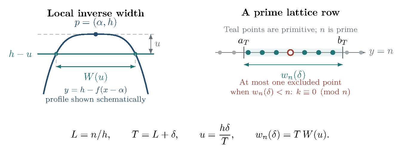
The theorem remains useful without a model formula for $f$. It measures the width of the graph at depth $L^{-2}$ and converts that width into a lower bound for the discrepancy. Infinite flatness implies, for every $N$, a lower bound $W(u)\gg_N u^{1/N}$ and recovers Proposition 29.1. A specified modulus yields a specified slowly varying factor. Figure 9 illustrates the passage from this local width to the new primitive points on a supporting row.

30.5 Model flatness profiles and what they do not determine

For illustration, suppose the two-sided local graph satisfies $$f(s)\leq C\exp\!\left(-\frac a{|s|^\beta}\right), \qquad a,\beta>0,$$ for sufficiently small nonzero $s$. Then $$W(u)\geq 2\left(\frac a{\log(C/u)}\right)^{1/\beta},$$ and (30.7) gives, along arbitrarily large prime-row contact scales, $$\max\{|E_B(L)|,|E_B(L+L^{-1})|\} \gg_{B,a,\beta}\frac L{(\log L)^{1/\beta}}.$$(30.8) If the graph has matching upper and lower estimates of this form, the row width itself has this order. This does not prove that the full discrepancy has exactly this order; other rows and other supporting directions can contribute.

Other infinitely flat local profiles give different slowly varying factors. For example, the symmetric model $f(s)=\exp[-\exp(|s|^{-\beta})]$ gives a row width of order $L/(\log\log L)^{1/\beta}$. The model $$f(s)=\exp[-(\log(1/|s|))^\gamma],\qquad\gamma>1,$$ gives a width of order $$L\exp[-(2\log L)^{1/\gamma}].$$ These are convex for sufficiently small $|s|$ and illustrate local possibilities. They are not asserted here to be the precise profiles of a hyperbolic torus norm ball.

For a strictly convex body, $W(u)\to0$. Consequently the single-row argument with a microscopic scale increment yields a quantity $o(L)$, although it can exceed every fixed power $L^{1-\varepsilon}$. It neither proves a literal $\Omega(L)$ lower bound nor distinguishes an $O(L)$ global remainder from an $O(L\log L)$ remainder. Its role is to quantify one geometric obstruction, rather than to identify the entire sharp remainder.

30.6 An exact row diagnostic and its precision requirements

For an arbitrary positive integer $n$ and a row interval $[a,b]$, the primitive count is exactly $$\#\{k\in\mathbb Z\cap[a,b]:\gcd(k,n)=1\} =\sum_{d\mid n}\mu(d) \left(\left\lfloor\frac bd\right\rfloor -\left\lceil\frac ad\right\rceil+1\right).$$(30.9) In particular, it equals $$(b-a)\frac{\varphi(n)}n+O(2^{\omega(n)}).$$ The formula includes endpoints exactly. For prime $n$ and $b-a<n$, the simpler absolute-error comparison with $b-a$ used above applies.

One can therefore record the local statistic $$J_n=P_{B,n}(n/h+h/n),\qquad P_{B,n}(T)=\#\{k\in\mathbb Z:\gcd(k,n)=1,\ (k,n)\in TB\},$$ at prime $n$. Since $L=n/h$ and $h/n=L^{-1}$, the proposition gives $$J_n=(L+L^{-1})W\!\left(\frac h{L^2+1}\right)+O(1).$$ This statistic needs no estimate of $\operatorname{Area}(B)$; it tests the local flatness mechanism directly. It does require a verified lattice-rational supporting normal at an irrational radial point. Finding such a direction is a separate geometric step and is not automatic for an arbitrary fixed surface.

The height $h$ must also be known accurately. If $\widetilde h=h+e$ and $|e|\le h/2$, then the exact contact-scale error satisfies $$\left|\frac n{\widetilde h}-\frac nh\right| =\frac{L|e|}{|h+e|}\le\frac{2L|e|}{h}.$$ Resolving the window of width $L^{-1}$ therefore requires a height error small compared with $hL^{-2}$. Using a larger window relaxes this requirement but changes the depth sampled by (30.5) and increases the background main-term increment. The local statistic is consequently complementary to a global main-term-free discrepancy diagnostic; it does not replace one. In an implemented row count, the floor and ceiling operations in (30.9) also require certified endpoint comparisons with the relevant integers, or an explicit range of possible counts when those comparisons are unresolved. Agreement at two working precisions does not certify a transcendental height or endpoint.

30.7 A trace diagnostic: historical report and new full campaign

The count here is $N_X(L)$ for unoriented essential simple closed geodesics on a once-punctured torus, with the convention $N_X(L)=\#\{\gamma:\ell_\gamma\le L\}$. Each primitive pair $(p,q)\in\mathbb Z^2$ is identified with $(-p,-q)$, so this is half the signed primitive-vector count for the corresponding norm ball. A positive trace triple satisfies $$x^2+y^2+z^2=xyz,\qquad x,y,z>2,$$ and a Farey edge replaces $z$ by $xy-z$. The identification of Farey regions with simple curves and this edge relation are described in [112, Sections 1–2]. For the experiment take the reduced triples $$(x,y,z)=(3,3,3),\qquad (x,y,z)=\left(\frac52,\frac{10-\sqrt{11}}2,4\right).$$(30.10) The first is the modular torus; the second is an asymmetric example. Both satisfy $2<x\le y\le z\le xy/2$.

Assign the root curves the slopes $(1,0)$, $(0,1)$, and $(1,1)$, respectively. The three open sectors between these roots enumerate every other unoriented primitive slope once by Farey mediants. In the negative-slope sector use the signed endpoints $(1,0),(0,-1)$; the other two sectors have endpoints $(1,0),(1,1)$ and $(0,1),(1,1)$. Canonical representatives have $q>0$, with $(1,0)$ as the only representative at infinity. Sector endpoints are counted only as roots. After introducing an outward trace $c\ge\max(a,b)>2$, the two new traces are $ac-b$ and $bc-a$, both strictly larger than $c$. Therefore pruning a sector when its new curve exceeds the cutoff does not omit shorter descendants. Equal traces are retained with their curve multiplicities; they are not deduplicated. The hyperbolic length associated with trace $x$ is $2\mathop{\mathrm{arcosh}}(x/2)$.

To avoid overflow the computation uses logarithmic traces. If $u_a=\log a$, $u_b=\log b$, and $u_c=\log c$, then $$\log(ab-c)=u_a+u_b+ \log\bigl(1-\exp(u_c-u_a-u_b)\bigr).$$ On the chosen outward edges the subtracted ratio is at most $1/2$, so this computation avoids catastrophic cancellation. The supplied draft describes extended-precision arithmetic for this recursion and double precision for sorting the resulting lengths. That reported implementation was not included in the supplied materials. Both maintained replacement calculations below use binary64 logarithmic recursion, with separate multiprecision trace checks. Neither provides an interval certificate of every event location.

30.8 A recent qualification of irrational flatness

Doan–Li–Nguyen’s preprint [113], version 3 dated 9 October 2026, states a Diophantine refinement of the irrational flatness statement. Its Theorem 4.7 on page 23 states that infinite graph-flatness holds precisely when the exponential rational-approximation exponent vanishes; superexponentially approximable irrational directions can have graph-flatness order only one. In slope coordinates the relevant vanishing criterion is $\limsup_j(\log q_{j+1})/q_j=0$, where $q_j$ are continued-fraction denominators; Lemma 4.8 on pages 25–26 specifies the slope-coordinate normalization. The proposed local convexity mechanism is that a nearby rational corner can remain visible at a much smaller spatial scale than its exponentially small angle.

We have checked these statements against that pinned version, but have not independently audited its flatness proof or its global counting assertions. None is used as a proved input above. In particular, Propositions 29.1 and 30.2 retain their explicit flat-point hypotheses, and Proposition 30.1 uses only strict convexity. The preprint also continues to list the McShane–Rivin $O_X(L\log L)$ bound as the cumulative counting benchmark; its multiplicity estimate concerns exact length levels, a different question.