9 Volume Hessians, finite elements, and computational complexity

9.1 The cotangent form and the correct deformation coordinates

Let $\mathcal T$ be a finite, connected, consistently oriented simplicial triangulation of a closed disk, with interior vertices $I$ and nonempty boundary vertex set $B$. Each triangle has three distinct vertices. For a piecewise affine function $v$ on a geometric realization, integration over each triangle gives $$\int_{|\mathcal T|}|\nabla v|^2\,dA =\sum_{e=ij}w_e(v_i-v_j)^2=v^TLv, \qquad w_e=\frac12(\cot\alpha_e+\cot\beta_e).$$(9.1) Here each undirected edge is counted once, $\alpha_e,\beta_e$ are its opposite angles, and the second term is omitted on a boundary edge. To check the normalization, the off-diagonal stiffness entry on a triangle is $\int_T\nabla\phi_i\cdot\nabla\phi_j\,dA=-\tfrac12\cot\alpha_k$ for its barycentric functions. Row sums vanish, giving the displayed edge form. This is the cotangent network of the finite element and electrical interpretations [119].

The energy is nonnegative on every geometric mesh, even if some edge weights are negative. The additional condition for nonnegative interior conductances is local Delaunayness: $$w_e=\frac{\sin(\alpha_e+\beta_e)} {2\sin\alpha_e\sin\beta_e}\ge0 \quad\Longleftrightarrow\quad \alpha_e+\beta_e\le\pi.$$(9.2) Grounding the boundary makes $L_{II}$ positive definite; a trianglewise proof, including zero Delaunay weights, is given below. When the relevant weights are nonnegative, solving its Dirichlet problem is solving Kirchhoff’s equations. Boundary-to-boundary edges do not enter this Dirichlet system; positivity of their weights is an additional condition if the full matrix is used in a different boundary problem.

Now prescribe the sums $\Delta_e=\alpha_e+\beta_e\le\pi$ opposite interior edges, and prescribe the single opposite angle on each boundary edge. An angle structure assigns positive corner angles, with sum $\pi$ in every triangle and these prescribed edge sums. Assume this positive angle domain is nonempty. For planar realization the data also satisfy $\sum_{e\ni i}(\pi-\Delta_e)=2\pi$ at each interior vertex; the left-hand side is its total angle in every such angle structure. If the intended planar boundary is strictly convex, impose also $$0<\kappa_b:=\sum_{t\ni b}\alpha_{t,b} =\sum_{e\ni b}(\pi-\Delta_e)-\pi<\pi \qquad(b\in B).$$ Here $\Delta_e$ denotes the single prescribed opposite angle on a boundary edge. These boundary inequalities are needed for the convex polyhedral interpretation; the Hessian identities below already hold on the abstract positive angle domain. Positive feasibility alone does not impose convexity of the developed boundary. Orient the triangles consistently. If a corner $c$ is opposite the directed edge $i\to j$, set $$\alpha_c(u)=\alpha_c^0+u_i-u_j,\qquad u|_B=0.$$(9.3) These are leading–trailing coordinates, not logarithmic scale factors. Triangle sums telescope; increments opposite a shared edge cancel. To prove that they parametrize the entire affine solution space, first use the edge equations to leave one signed increment per interior edge. The triangle equations are then the incidence equations of the connected dual graph of faces, of rank $N_T-1$. If $E_{\mathrm{int}}$ is the number of interior edges and $N_T$ the number of triangles, Euler’s formula gives $$\dim T\mathcal A=E_{\mathrm{int}}-N_T+1=|I|.$$ The coordinate map is injective: if every corner increment vanishes, $u$ is equal across every edge, hence constant by connectedness, and the boundary condition makes it zero. It therefore has the required dimension. This argument uses the disk topology; on an annulus extra period directions can remain. In these coordinates the positive domain is $$\Omega=\{u\in\mathbb R^I:\alpha_c^0+u_i-u_j>0 \text{ for every corner }c\}.$$ It is nonempty, open, convex, and bounded. Positivity and the triangle sums imply $\alpha_c<\pi$; injectivity transfers this boundedness to $u$.

Let $\Lambda'(a)=-\log(2\sin a)$ be the Lobachevsky derivative and put $\mathcal V(\alpha)=\sum_c\Lambda(\alpha_c)$. At a geometric configuration this is the sum of the volumes of the ideal tetrahedra obtained by adjoining the vertex at infinity to the planar triangles. Rivin’s variational principle uses this concave functional to impose geometric closure [120; 37]. Existence and realization statements require their geometric hypotheses; prescribed Delaunay data and flat convex disks are treated separately in [121, Theorems 1.6 and 4.11]. The differential identities below do not assume that every point of $\Omega$ already has a global planar realization.

Consequently $\mathcal V$ is strictly concave on $\Omega$. An interior critical point, if it exists, is the unique maximum there and also a maximum on its closure by continuity. Its equations $H_i=1$ kill dilation holonomy. The separately imposed total-angle equations kill rotational holonomy; convex boundary data and a global realization argument supply the polyhedral interpretation. Strict concavity alone does not place the maximizer in the interior.

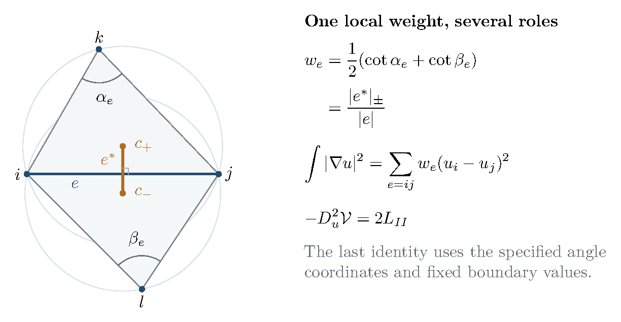
For a true interior edge with $0<\Delta_e<\pi$, the weights satisfy $$w_e=\frac{\sin\Delta_e}{2\sin\alpha_e\sin\beta_e} \ge\cot(\Delta_e/2)>0.$$(9.5) Thus positivity holds throughout the angle domain, before the angles close to form a geometric mesh. At $\Delta_e=\pi$ the weight is zero; at a geometric polyhedral realization such a diagonal subdivides a flat face. A zero abstract weight by itself asserts no embedding. The kernel proof also shows that these zero weights create no extra grounded zero modes. The finite element interpretation as an actual planar mesh applies at realization, whereas the Laplacian identity and positive-network interpretation already apply to the intermediate angle structures. Newton’s equation is precisely $$2L_{II}(\alpha(u))\,\delta u=\log H(u).$$(9.6) Figure 3 summarizes the local edge weight and its finite-element and volume-Hessian interpretations.

9.2 Boundary response, Schur complements, and a Gaussian factor

For the finite element network, eliminating the interior voltage gives $$v_I=-L_{II}^{-1}L_{IB}v_B,\qquad \mathcal N=L_{BB}-L_{BI}L_{II}^{-1}L_{IB}.$$(9.7) The matrix $\mathcal N$ maps boundary voltages to boundary currents; it is the discrete Dirichlet-to-Neumann operator. Indeed, minimizing $v^TLv$ at fixed $v_B$ gives the first equation and the minimum $v_B^T\mathcal N v_B$. It follows that $\mathcal N$ is positive semidefinite and that its kernel consists exactly of boundary constants. Grounding one boundary vertex, or working modulo constants, makes it positive definite. This energy statement allows signed boundary weights; the full passive resistor interpretation requires nonnegative weights.

The same elimination appears in volume response. For a smooth function with a nondegenerate local maximum at the origin, write $$\mathscr V(x)=V_0-\tfrac12x^TKx+O(|x|^3),\qquad K>0,$$ and let $Px$ be selected linear observables. These are geometric boundary data only when the model supplies that identification; they are not the fixed coordinates $u|_B=0$. The implicit-function theorem gives the local maximizing branch $x(j)=K^{-1}P^Tj+O(|j|^2)$. Thus perturbation by a source $j$, or restriction to $Px=b$, gives the local expansions $$\begin{aligned} \max_{x\text{ near }0}\{\mathscr V(x)+j^TPx\} &=V_0+\tfrac12j^T\chi j+O(|j|^3), &\chi&=PK^{-1}P^T,\\ \max_{\substack{Px=b\\x\text{ near }0}}\mathscr V(x) &=V_0-\tfrac12b^T\chi^{-1}b+O(|b|^3), \end{aligned}$$ where the second formula assumes $P$ has full row rank, so $\chi>0$. The first is the response to a source; the second fixes its conjugate variable. They are related by a Legendre transform. In the planar problem $K=2L_{II}$; in the Dehn filling problem, the same algebra gives (16.7) and (16.8). This identifies an exact common operation without identifying their different spaces of boundary data.

More generally, split $x=(y,z)$ and eliminate $y$. The effective quadratic form is $$K_{\mathrm{eff}}=K_{zz}-K_{zy}K_{yy}^{-1}K_{yz},\qquad \det K=\det K_{yy}\det K_{\mathrm{eff}}.$$(9.9) For $\hbar>0$, completing the square gives the exact real Gaussian identity $$\int_{\mathbb R^{\dim y}} e^{-\frac1{2\hbar}(y,z)^TK(y,z)}\,dy =\frac{(2\pi\hbar)^{\dim y/2}}{\sqrt{\det K_{yy}}} e^{-z^TK_{\mathrm{eff}}z/(2\hbar)}.$$(9.10) Thus elimination in the Dirichlet problem, reduction of the classical boundary action, and its leading Gaussian integration use the same Schur complement. An oscillatory or complex phase requires the specified contour and determinant branch, as in the later quantum calculations. The finite-dimensional identity does not supply those analytic data or identify an entire quantum invariant by itself.

There is also a combinatorial formula for the planar determinant. Let $\mathfrak F_B$ be the spanning forests of the weighted graph in which each component contains exactly one boundary vertex. Then $$\boxed{\det(-D_u^2\mathcal V) =2^{|I|}\sum_{F\in\mathfrak F_B}\prod_{e\in F}w_e.}$$(9.11) To prove it, write $L_{II}=C_I\operatorname{diag}(w_e)C_I^T$, where $C_I$ is the incidence matrix with boundary rows removed. Cauchy–Binet expands its determinant over $|I|$-edge subsets. An incidence minor is $\pm1$ exactly for a forest rooted at $B$, and zero otherwise. This rooted-forest formula expresses the local Gaussian determinant in geometric conductances. It is a deduction from the Hessian identity and finite-dimensional linear algebra. The incidence-minor identity holds for real signed weights as well; in the Delaunay Dirichlet problem its contributing weights are nonnegative. Zero-weight edges contribute zero terms, and strictness of $L_{II}$ makes the total positive.

9.3 Why the nonlinear iteration needs a barrier

A fast linear solve does not by itself bound the number of Newton steps. In particular, $-\mathcal V$ is not uniformly self-concordant: near a vanishing angle, its entropy-like behavior makes the normalized third derivative unbounded. The companion study supplies a more useful estimate involving the barrier $$F(\alpha)=-\sum_c\log\sin\alpha_c.$$(9.12) The coefficient $\csc^2\alpha_c$ occurs in both $D^2F$ and $D^3\mathcal V$, but these are tensors of different order. The precise relation needed for optimization is the following inequality.

All derivatives and inverse local norms in the following argument are taken on the intrinsic affine angle space, after linear dependencies have been removed. The parameter bound $m$ belongs to $F$; $F-t\mathcal V$ is a standard self-concordant objective, not a barrier claimed to have that same parameter.

Write $\Phi_t=F-t\mathcal V$ and $H_t=D^2\Phi_t$. A nonempty positive angle domain has compact closure in angle coordinates. Since $F$ tends to infinity at its relative boundary while $\mathcal V$ is continuous on the closure, $\Phi_t$ has a unique interior minimizer $x_t$. The zero-dimensional case is vacuous. If $\mathcal V^*$ denotes the maximum on the closed feasible domain, then $$\mathcal V^*-\mathcal V(x_t)\le\frac m t.$$ Indeed, concavity of sine gives $0\le\sin\beta_c\le\sin x_c+\cos x_c(\beta_c-x_c)$, hence $DF(x)[\beta-x]\le m$ even for a closed feasible $\beta$ with zero angles. At $x_t$, use $DF=tD\mathcal V$ and concavity of $\mathcal V$. This argument does not assume that its closed maximizer is positive.

For a finite iterate $x$, define the Newton decrement $\lambda_t(x)=\|D\Phi_t(x)\|_{H_t(x)^{-1}}$. If $\lambda=\lambda_t(x)<1$, self-concordance gives $r:=\|x_t-x\|_{H_t(x)}\le\lambda/(1-\lambda)$. For completeness, put $d=x_t-x$. Along the segment the one-direction Hessian bound is $D^2\Phi_t(x+s d)[d,d]\ge r^2/(1+s r)^2$. Integrating and using stationarity at $x_t$ gives $-D\Phi_t(x)[d]\ge r^2/(1+r)$, whereas dual Cauchy–Schwarz bounds the left side by $\lambda r$. Moreover, $H_t\succeq D^2F$ implies $$t\|D\mathcal V(x)\|_{H_t^{-1}}\le\sqrt m+\lambda.$$ Concavity at $x$ now proves the finite-centering certificate $$\mathcal V^*-\mathcal V(x) \le\frac{m+(\sqrt m+\lambda)\lambda/(1-\lambda)}{t} \le\frac{17m}{12t}\quad\text{if }\lambda\le\tfrac14,\ m\ge1.$$

Here is an explicit short-step schedule. Start at $t_0>0$ with $\lambda_{t_0}(x_0)\le1/4$, increase $t$ by $1+1/(20\sqrt m)$, and take one full Newton step for the new objective. With $\delta=(t'-t)/t$, the identities $$D\Phi_{t'}=(1+\delta)D\Phi_t-\delta DF, \qquad H_{t'}\succeq H_t$$ bound the new decrement before the step by $(1+\delta)/4+\delta\sqrt m\le5/16$. The standard self-concordant Newton estimate makes the step feasible and bounds its new decrement by $(\lambda/(1-\lambda))^2\le25/121<1/4$. Stopping when $t\ge17m/(12\varepsilon)$ therefore gives $$O\!\left(\sqrt m\log\max\left\{e,\frac{m}{t_0\varepsilon}\right\}\right) \quad\text{Newton steps to volume gap at most }\varepsilon.$$(9.14) This bound assumes the stated initial centering; it does not pay for finding or centering a feasible point. The underlying Newton estimates are described in [122, Chapter 11] and the authors’ lecture notes [123]. They apply here to the specified barrier schedule, not to unrestricted plain Newton iteration.

In the disk coordinates the Hessian of $F-t\mathcal V$ is again a grounded planar Laplacian, now with interior conductances $$2t w_e+\csc^2\alpha_e+\csc^2\beta_e.$$ An energy-norm tolerance makes the inexact version concrete. At the new parameter, let $d_N=-H^{-1}g$, $\lambda=\|d_N\|_H\le5/16$, and suppose the computed step satisfies $\|d-d_N\|_H\le\lambda/100$. Put $\eta=\|d-d_N\|_H$ and $r=\|d\|_H$. Then $\eta\le1/320$ and $r\le101/320<1$. Hessian comparison and the integrated gradient remainder give $$\lambda_{\mathrm{new}} \le\frac{\eta}{1-r}+\frac{r^2}{(1-r)^2} \le\frac{10420}{47961}<\frac14.$$ The old dual-norm linear residual is at most $\eta$, the nonlinear remainder at most $r^2/(1-r)$, and conversion to the new dual norm costs at most $1/(1-r)$. This argument assumes exact gradient and Hessian evaluation apart from the stated solve error. Feasibility can also be checked directly: $\|d\|_H<1$ and $H\succeq D^2F$ imply $|d\alpha_c|<\sin\alpha_c\le\min\{\alpha_c,\pi-\alpha_c\}$ for every corner, so the new angles remain strictly between zero and $\pi$.

Nearly-linear Laplacian solvers provide relative energy-norm guarantees [124, Theorem 5.5]. With such tolerances maintained at every step, their combination with (9.14) gives the conditional randomized expected $\widetilde O(n^{3/2})$ arithmetic-work scale after centering, up to accuracy factors. Here $n=|I|+|B|$ is the full mesh vertex count; disk planarity gives $m=O(n)$ and $O(n)$ matrix entries. Success probabilities over all solves, coefficient precision and transcendental evaluations need their own controls. This is not a bit-complexity or floating-point stability bound. Finding a feasible point, centering it, and certifying the final geometric error are separate costs. The companion’s selected-input timings do not bound these additional tasks. The dense implementation described below follows the specified schedule, with numerical diagnostics; it does not implement a nearly-linear solver or certify floating-point error.

9.4 Flips connect the local matrix to mapping-class geometry

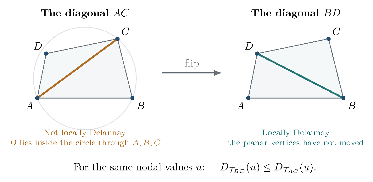
A diagonal exchange has two different roles. Among triangulations of the convex hull of a fixed planar vertex set, with fixed nodal values, Rippa’s theorem says that Delaunay triangulation minimizes the piecewise-linear Dirichlet energy; in matrix terms $L(\mathcal T_D)\preccurlyeq L(\mathcal T)$ [125]. This is an ordering of quadratic forms for the same geometric data. It does not assert monotonicity of hyperbolic volume along an arbitrary sequence of topological flips. Figure 4 illustrates the comparison for one fixed Euclidean quadrilateral.

For a connected orientable finite-type marked surface admitting an ideal triangulation, with at least one marked point on every boundary curve, the graph of ideal triangulations and diagonal exchanges is instead a coarse geometric model of its mapping class group. For orientation- preserving classes and isotopies fixing the marked points individually, the action is proper and cocompact, and an orbit map is a quasi-isometry [126, Section 2.1, Lemma 2.3]. For a closed oriented surface of genus at least two, the pants graph is a different model, quasi-isometric to Teichmüller space with its WP metric. In this setting Brock compares the convex-core volume of the quasi-Fuchsian manifold with conformal ends $X,Y$ to $d_{\mathrm{WP}}(X,Y)$, with topology-dependent multiplicative and additive constants [127, Theorems 1.1–1.2]. For pseudo-Anosov monodromy on the same closed surface, mapping-torus volume and WP translation distance are comparable with topology-dependent multiplicative constants [128, Theorem 1.1]. The flip graph and pants graph have different metric roles.

There is a direct volume estimate when a flip sequence gives a layered ideal triangulation of a hyperbolic mapping torus with $N$ tetrahedra: straightening gives $\operatorname{Vol}(M)\le Nv_3$, where $v_3$ is the volume of the regular ideal tetrahedron. This does not require the given triangulation to have positive geometric shapes; signed straightened volumes still have absolute value at most $v_3$. It connects a combinatorial decomposition length to three-dimensional volume. Comparing it further to WP geometry requires a theorem for the same surface and boundary conventions, rather than transferring the closed-surface theorem silently to a punctured surface.

9.5 The three-manifold extension and the remaining questions

The Casson–Rivin program uses the same ideal-tetrahedron volume and the same angle-sum constraints [37]. Its local Hessian is still a cotangent quadratic form. For leading–trailing edge variables $y_e$, put $p_\alpha=y_e+y_{e'}$ for the pair of opposite tetrahedron edges carrying $\alpha$, and cyclically for $\beta,\gamma$. Then $$-D^2\mathcal V =\sum_t\left[ \cot\alpha_t(dp_\gamma-dp_\beta)^2 +\cot\beta_t(dp_\alpha-dp_\gamma)^2 +\cot\gamma_t(dp_\beta-dp_\alpha)^2\right].$$(9.15) This displays the Euclidean cusp-link triangle inside the second variation. But a square now involves sums of opposite-edge variables, and the assembled matrix need not have nonpositive off-diagonal entries or be diagonally dominant. Additional peripheral directions and removal of linear dependencies must also be included in a full coordinate system. The planar positive-Laplacian solver conclusion therefore does not transfer automatically to arbitrary three-manifold triangulations. The trianglewise barrier estimate does transfer, because it survives affine restriction.

For an ideal triangulation of an orientable compact three-manifold whose nonempty boundary is a union of tori, a positive angle structure critical for volume on the full angle space supplies the complete hyperbolic metric on its interior, by the Casson–Rivin theorem [37, Theorem 1.2]. The angle space has triangle sums $\pi$ and edge sums $2\pi$; full criticality includes the peripheral directions. Edge variations alone do not impose completeness. A boundary maximizer need not realize the chosen triangulation by positive ideal tetrahedra. Optimization on a given angle polytope therefore does not solve the problem of finding a suitable geometric triangulation or yield a polynomial-time geometrization algorithm.

The finite element comparison also does not identify its real symmetric Hessian with the alternating WP form. The exact links established here are the volume Hessian, its inverse response, its Schur complement, and its Gaussian determinant. A continuum limit relating appropriately renormalized polyhedral functionals to a WP potential would require geometric convergence, a specified normalization, and control of second variations. This is a natural question, not a theorem asserted here. Likewise, in three dimensions it remains useful to ask for an effective bound on the smallest angle at an interior maximum in terms of the number of tetrahedra and a quantitative feasible margin. Such a bound would connect variational existence to numerical certification and complexity. These questions describe how the computational strand can extend the monograph’s variational and semiclassical program.

9.6 Reproducible computational examples

The Section 9 reproduction guide connects these formulas to a fixed $3$ by $2$ integer-coordinate grid, triangulated into twelve right-isosceles triangles with two interior vertices. At its geometric angle assignment, $$L_{II}=\begin{pmatrix}4&-1\\-1&4\end{pmatrix},\qquad K=-D_u^2\mathcal V=\begin{pmatrix}8&-2\\-2&8\end{pmatrix},\qquad \det K=60.$$ An independent rational finite-element assembly gives this matrix. Exhaustive boundary-rooted forest enumeration gives fifteen unit-weight terms, so (9.11) gives $2^2\cdot15=60$. Eliminating the first variable of $K$ leaves $K_{\mathrm{eff}}=15/2$, and $8(15/2)=60$. Prescribing the electrical boundary voltage $v=x/3$ gives interior values $1/3,2/3$ and energy $2/3$. These are exact finite identities for the named fixture, separate from the general proofs above.

The maintained numerical operators assemble angle increments, gradients, Hessians and boundary response. The experiment driver also compares the binary64 volume with $12G$, where $G$ is Catalan’s constant, and an off-origin Hessian with independent numerical differentiation at 50-digit working precision. The result record states source and input hashes, methods, residuals and tolerances. These numerical comparisons are not interval enclosures.

The worked computational companion and complete reproduction archive provide the input, runnable code and environment requirements. The grid has zero-weight square diagonals and is therefore non-strict Delaunay. Off-origin angles belong to the abstract domain; their geometric closure is not asserted.

The separate barrier examples exercise the dense affine-angle solver. It accepts a supplied positive angle vector and independent tangent columns, performs separately budgeted initial centering, and then follows the short-step parameter schedule above. Every accepted point records its parameter, Newton decrement, angle margins, linear-solve residual and numerical conditioning. Rejected domains, failed steps and exhausted budgets remain unsuccessful outcomes; angles are not clipped into the domain. The reported finite-gap estimate is evaluated in binary64 arithmetic and is not an interval certificate.

The barrier experiment driver compares the computed endpoints with independent multiprecision volume references and checks the recorded path and stopping conditions. The fixed cases are the full single-triangle angle simplex with its maximum at the regular ideal tetrahedron, an asymmetric rectangular disk, and a two-triangle affine slice with one flat triangle at its closed maximum. Its result record separates initial-centering work from path steps, and its reproduction archive contains the actual code, inputs and environment requirements. These finite examples do not establish a scaling law. A nearly-linear solver, a certified relative energy-error bound, a peripheral-holonomy solver and a global realization certificate remain outside this implementation. The claim ledger distinguishes this numerical coverage from the general proofs, external theorem inputs and open questions.